Legacy GPS receiver in Matlab
When people say GPS they usually unknowingly mean GNSS (Global Navigation Satellite System ). GPS is just one of GNSS out there and is run by the Americans. The other big players on the block are BeiDou by China, Galileo by Europe, and GLONASS by Russia.
The orbits of these satellites hang out at around 20,000 km above the Earth, midway between the center of the Earth and the geostationary satellites such as TV satellites and the like. So they are a long way away. GPS has to have the sweetest orbit of the bunch as the satellite constellation repeats almost exactly every Earth’s rotation which is called a sidereal day or about four minutes less than 24-hour. Wikipedia has a really nice animation of the GNSS satellites as can be seen below…
 Comparison satellite navigation orbits
You can see the international space station (ISS) almost scrapes the earth in comparison to the GNSS satellites.
I have done some bits and pieces with GNSS; mainly finding novel ways to use raw data from GNSS receivers. The raw data consists of observables and navigation data. Observables are the measurements the GNSS makes and navigation data is information sent from the satellite. Contrary to what some people think GPS/GNSS receivers are just that they don’t transmit anything to the satellites. This brings up one issue I have about talking to people about “GPS”, just because almost everyone these days carries a “GPS” receiver on them in their phone they think it’s simple and know everything about it; it’s not. It’s truly quite an amazing technological feat costing billions of dollars and continued expensive maintenance to keep it running every day, day in day out (how-much-does-gps-cost). Even in 1979 the Americans spent over $4 billion on it before most people would’ve even heard about it ( initial GPS cost ). The complexity of how it all works is jaw-dropping and over the years continues to mature, evolve, and try to produce ever better positions solution.
All but GLONASS use CDMA (Code Division Multiple Access). However it looks like even GLONASS is going to get into the CDMA game. GLONASS has historically used FDMA and a system I know relatively little about so I’ll stick to CDMA for the rest of this document.
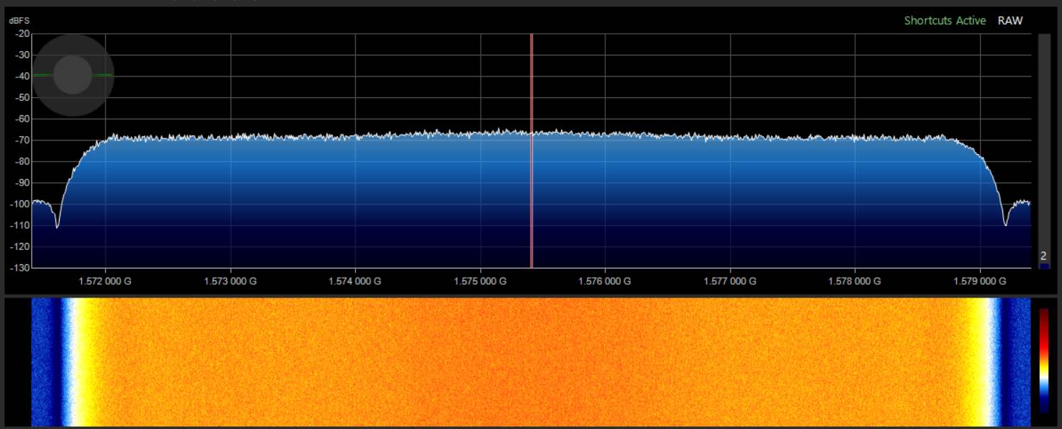
I’m sure I haven’t been the only one to turn on an SDR (Software Defined Radio), point it to 1575.42 MHz (the traditional place GPS hangs out at) with as much bandwidth as the SDR can cope with and see nothing…
 Spectrum of L1 GPS signal band: Where is it?
That’s a disappointment 7 MHz of bandwidth and you can’t see a signal. Actually there is a lot going on in this band.
Navipedia is a great resource for the GNSS curious. Here is a band plan for GPS around 1575.42 MHz (circa 2020) from Navipedia, this band is called L1…
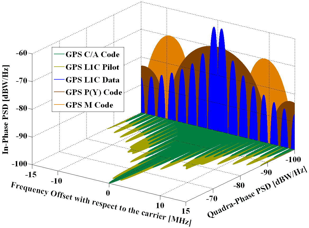 L1 GPS band plan courtesy of Navipedia signal plan
So from GPS alone there are five signals in this band. Then maybe there are 10 GPS satellites visible at my location using the same band at the same time. Galileo and BeiDou also use these frequencies so add another four signals for them and maybe a couple of signals for the Japanese and you’ve got a very busy band indeed.
Let’s look at the legacy GPS C/A L1 signal. It uses DSSS (Direct Sequence Spread Spectrum). DSSS uses a known pseudorandom number ([PRN]) which for me I’m going to define of as consisting of a finite number of -1s and +1s, seemingly random but the receiver knows the sequence and can reproduce it itself. That being the case the following figure is what the satellite is transmitting for the C/A L1 signal.
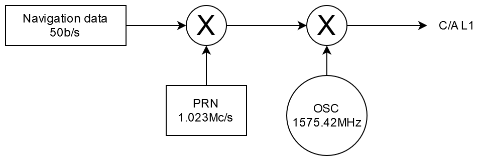 C/A L1 signal being transmitted by the satellite
Everything is driven by a single 10.23 MHz clock; it’s multiplied by 154 to get 1575.42MHz for the carrier and divided by 10 to get the chip rate of the PRN of 1.023Mc/s. The PRN has a length of 1023 and every 20th PRN causes the 50b/s needed for the navigation data. The only difference between a bit and chip is that a chip doesn’t really contain any unknown data as the sequence is already known. So if we ignore the navigation data which we can as its it so slow compared to the PRN, effectively we have a BPSK transmitter with a symbol rate of 1.023Mb/s at 1575.42MHz, this is why the C/A signal (the figure below) looks like BPSK and its main lobe is about 2.046 MHz.
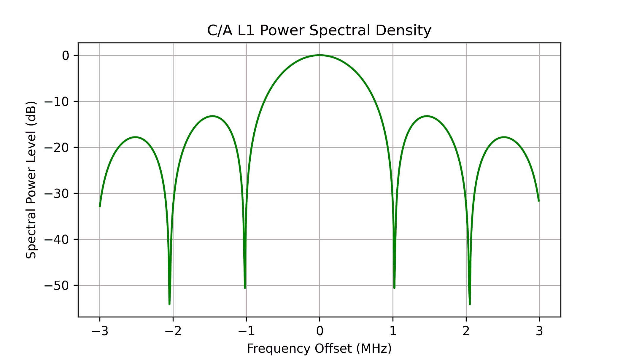 C/A L1 spectrum of the transmitted C/A L1 signal
At the receiver, as the PRN is already known, if we mix the PRN with the incoming signal such that they align, then all the spreading caused due to the PRN being injected into the transmitter will be removed and we will get a very narrow or despreaded signal with just enough bandwidth for the 50b/s navigation data. This despreading causes the signal to pop up above the noise floor so it can be seen.
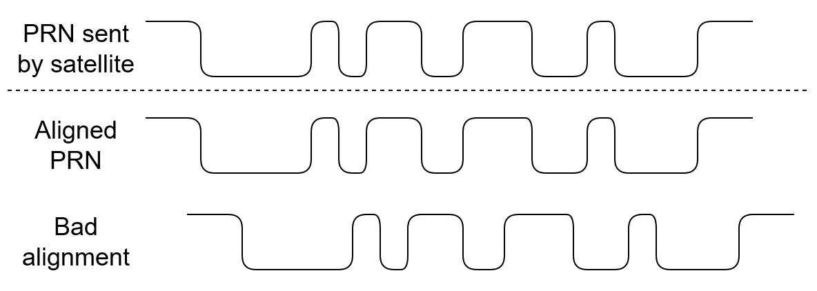 Good and bad alignment of the local PRN signal with the received one
As well as aligning the PRN with the incoming signal we also have to do the not so fun part of making sure our receiving oscillator has the exact same frequency of that of the transmitter, i.e. 1575.42 MHz. If we don’t get this frequency exact then the PRN we are receiving will rotate and the correlation (mixing then sum, integration or whatever you want to call it) that we will be doing will not always be constructive. Imagine the points starts out on the real axis with +1 pointing to the right for the first 50% of the correlation and then suddenly rotate such that for the last 50% of the correlation +1 now points to the left; this means that when we correlate this with the PRN, half will be constructive, half will be deconstructive and will get nothing; the following shows an example of this…
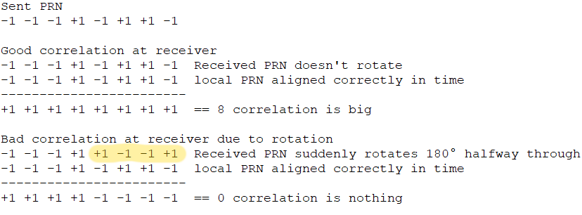 Correlation example
So that means we have to simultaneously find the correct PRN alignment in time as well as the correct carrier frequency offset to present the incoming signal form rotating too fast. When we do this we should see a signal.
Why Matlab?
Matlab/Octave I find handy for exploring and learning purposes. It’s good for quick mockups and testing out ideas. Code wise it can get rather unwieldy quite quickly, it’s not strongly typed and you can get some subtle bugs if you’re not careful. I find it quite difficult going back to Matlab code I’ve written in the past and usually I don’t. Usually what I do is explore in Matlab to gain knowledge, if anything really has to be put into a program I’ll move it into something like C++ after I have a better understanding of it. So for this little project I am really just getting a feel for what GPS and maybe Galileo signals are like. I doubt I’ll ever put anything of this project’s Matlab code into C++ as you can buy GNSS modules off-the-shelf to do anything I can think of at the moment. However, if I find I can’t get a GNSS module that does what I want it to do, well then things might change.
First steps
First we need to record the RF signal which I have already done using the RSP1 SDR receiver, a 5 m USB extension cord, a Bias tee made with some scrap PCB, a LiPo battery, and an off-the-shelf active GPS antenna for the L1 band ( 1575.42 MHz ). I used SDRuno to record it with a setting of 8 MHz and a gain as high as it would go. I recorded about 19 seconds which was about 595 MB. I couldn’t figure out how to play back the recording with SDRuno but I did manage to play it back with SDR# and looked and sounded normal. It recorded with a WAV file extension name so I assumed it was a standard stereo recording albeit with a really high sample rate and instead of stereo assumed it would be one channel for the real and the other one for the imaginary. I assume it’s using 16 bit format for the WAV file. Usually front-ends of GPS receivers have a very low bit rate of just a few bits so most of these 16 bits aren’t necessary and are making the wav file unnecessarily large.
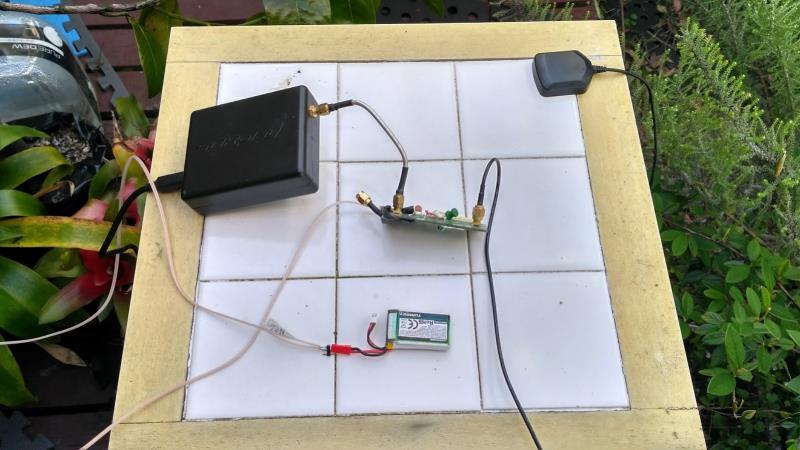 Hardware setup for the 19s recording
Getting the signal into Matlab is easy and is just the following code…
clear all;
close all;
clc;
amount_of_wav_file_to_use_in_seconds=1;
wav_file_offset_in_seconds=0;
c = 2.99792458e8;%speed of light m/s
chips_per_second=1023000;%C/A code chip rate
prn_len=1023;%number of chips till the code starts repeating
prns_per_second=chips_per_second/prn_len;
meters_per_prn=c/prns_per_second;

%read iq samples from wav file and get samplerate
filename='/home/jontio/Desktop/SDRuno_20201025_223133Z_1575409kHz.wav';
[~,Fs] = audioread(filename,[1,1]);%Fs is iq samplerate of wav file
samples = [1+wav_file_offset_in_seconds*Fs,amount_of_wav_file_to_use_in_seconds*Fs+wav_file_offset_in_seconds*Fs];
[y,Fs] = audioread(filename,samples);
y=y(:,1)+1i*y(:,2);

number_of_samples_per_chip=Fs/chips_per_second;
meters_per_sample=c/Fs;

%dont want the 1/2 issue
sympref('HeavisideAtOrigin',1);
So that was simple. I loaded 1 second here. Next we need something to generate the GPS PRN codes to allow us to have access to the signals, this too is incredibly simple as Dan Boschen has already done this for us and put it in a nice Matlab function that generates GPS C/A PRN codes, thanks. I haven’t checked but I assume the codes it generates are correct. Correlating the input signal with one PRN doesn’t produce a particularly good correlation compared to using the same PRN concatenated with itself again and again and again. However, as the navigation data signal inverts the PRN we can’t have too many of them else we have the problem that some of the PRNs end up becoming destructive if we cross the navigation bit boundary. Also the more we have the slower the initial signal acquisition becomes. It is possible to remove the navigation data once a signal has been acquired so we don’t get destructive correlation but we can’t do that yet. Anyway we still have to make a decision as to how many PRNs to concatenate, so for the time being let’s say 5. I’m not sure what to call this concatenated PRN thing but maybe “PRN block” or just block for simplicity to distinguish it between the usual PRN of length 1023. So our PRN block will have a length of 5115 while our PRN will have a length of 1023. We also have to choose a satellite. Looking at Orbitron I can see BIIRM-6 currently has PRN number 7 and is almost directly overhead so should be the strongest signal…
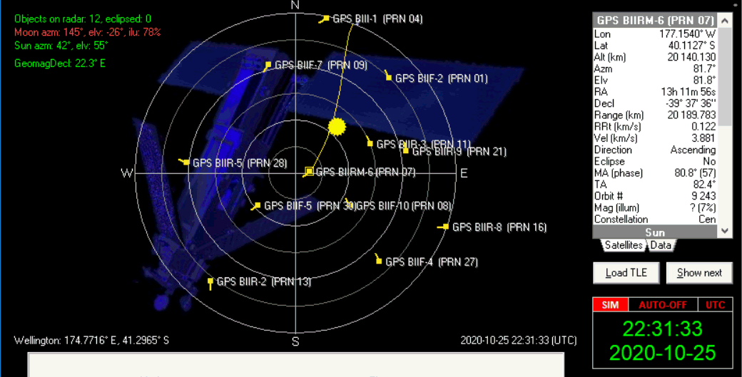 Satellites visible according to Orbitron
That being the case the following will make a PRN block of 5115 chips (5ms) for the satellite with PRN seven (sv=7). At 8M samples a second for the WAV file, prn has a length of 8000 samples and prn_block having five times the length will have 40,000 samples…
sv=7;
prns_per_correlation=5;
prn=2*(cacode(sv,number_of_samples_per_chip)'-0.5);
prn_len_in_samples=numel(prn);
prn_block=repmat(prn,[prns_per_correlation,1]);
prn_block_len_in_samples=numel(prn_block);
2D coarse search
This is an interesting problem and something that everyone seems to do as you can use FFTs and everyone loves FFTs. We have to find the correct chip alignment of the PRN with the incoming signal as well as the correct frequency offset between the SRD’s oscillator and the oscillator from the satellites transmitter once it reaches the receiver’s antenna. Initially we have no idea of either of the values so we have to search for them simultaneously. This search is quite CPU intensive even using tricky shortcuts.
In the following figure you can see the effect of correlation when you change the frequency of the incoming signal and the chip offset of the PRN…
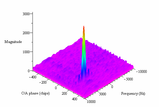 Correlation with respect to carrier frequency and PRN phase
Although this may offend mathematical purists who insist on subscripts for discrete values and using single symbols to describe something, here is what we’re doing when we are correlating to find the maximum peak for the 8 million samples per second recording I have made…
This function is a complex function. The absolute value of this or the magnitude of this function goes up when we get a better correlation; it shows how similar one thing is to another. is the chip offset in samples, is the frequency offset Hertz. Signal is the input signal, is what we are looking for in the signal, mod is the function that wraps numbers around such that remain within 0 to 7999, is time in discrete sample steps, is the square root of -1, is 3.14 ish.
will drop significantly even if we are out by a fraction of a chip. For our 8MHz sample rate one chip corresponds to about eight samples so if we move k one sample we are shifting the PRN block by 1/8th of a chip which is good enough so that we don’t miss the correlation peak. Frequency is less critical so say a frequency step of say 200 Hz should be fine. The frequency range to step through should be about 10 kHz to account for the Doppler effect of satellites as they hurtle towards or away from us but I’m not sure how accurate the RSP1’s oscillator is so maybe add another 10 kHz just to be safe. That means to search the entire 2D space we have different values for to try for and . For each pair of these values there are 40,000 things to sum together each of which requires 1 complex multiplication (forget about the exp one as it’s not significant for just 200 frequencies and can be precomputed), 8 operations for a complex multiply and accumulate (MAC) bringing us to a grand total of about 500,000,000,000 things to either add or multiply. Even if I’ve made a mistake somewhere with these back of the envelope calculations the number of multiplications and additions are huge. So let’s use FFT to do the hard work.
Fast circular correlation with FFT look something like the following…
What it returns is a vector of length 40,000 in our case where each entry corresponds to a different PRN block offset (different k). So it’s like the formula without the FFT but magically calculates every value of k hence why k is missing from the left-hand side of the formula. conj flips the imaginary component of every complex number, circshift circular shifts the first argument by the number given in the second argument, is element wise multiplication, FFT is the fast Fourier transform while is the inverse fast Fourier transform. This whole thing works because multiplication in the frequency domain is convolution in the time domain. We take our time domain signals put them into the frequency domain using FFT, take the conjugate of one of them which means we get correlation rather than convolution multiply them together in the frequency domain and move it back using to get the correlation. The circular shift thing in the frequency domain produces the frequency offset that we had to do in the time domain with the exp thing. If for some reason you want a fractional frequency shift then you can pad the signal with lots of zeros (a multiple of the length of the signal), take it into the frequency domain, shift it by an integer number, and then decimate it to get a length of the original signal. Anyway, I digress. One problem with this fast correlation is it returns five times the range over which we wish to find the maximum peak as the PRN block contains five concatenated PRNs. Here is a figure of the output of this function for good value of …
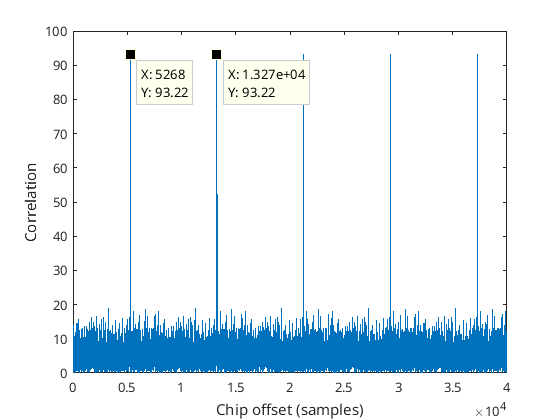 Circular correlation for whole of PRN block
You can see we get five peaks rather than one and they repeat about every 8000 samples. The method without the FFT we didn’t have to bother about these other peaks as we didn’t calculate anything beyond 8000 samples. So how many operations does this take? Let’s say the FFT takes operations for a discrete Fourier transform of length N. We have two initial FFTs to be done and after that we have to do 200 inverse FFTs. Before doing each inverse FFT we have to multiply 40,000 complex numbers together each requiring six real operations. That’s about 200(40,0006+540,000log2(40000)) or about 700,000,000 operations. So using these back of the envelope calculations using FFTs might be 1,000 times quicker, so yeah it’s worth it.
Sample rate of the ADC and Doppler Effect on the chip frequency
The coarse acquisition I’m proposing doesn’t alter the frequency of the chips, rather it just changes the phase of them en masse each PRN block correlation. This means during a correlation some chips may correlate better than other chips. What I’d like to know is how much of an issue is this?
It’s well known that the maximum Doppler shift for these GNSS satellites is about 5 kHz for the 1.57524 GHz signal or a radial velocity of about 929 m/s. So my search range of 20 kHz might be way overkill but anyway that’s what I’ve chosen and I’m not going back and rewriting all this. That’s an error of about 3ppm. For our PRN block of 40,000 samples that’s about 10% of a sample (1% of a chip) so I can probably get away with that.
I’m not sure what the SDR1’s ADC exactly operates at but let’s say it uses a crystal with a 20ppm accuracy. That’s 80% of a sample or 10% of a chip. Not so great but it will have to do for the meantime for the coarse acquisition. So it’s probably not going to be an issue for these PRN block correlations and we can also see that most of the frequency error comes from the SDR1’s ADC crystal.
If we wanted to be exact we would have to recalculate the prn block each time we altered the frequency in our 2D search. This would be a real hassle so it’s fortunate we can ignore this issue for the 2D search. However, once we finished the 2D search will have to figure out the frequency of the PRN.
Real life coarse 2D search using FFT
The following code example along with the previous two code examples will take a block of signal data from y and will plot a three-dimensional correlation figure for the given satellite. The 2D search itself in this code is only a couple of lines of code but still is quite a lot of work for the CPU.
signal=y(1:prn_block_len_in_samples);

max_freq_offset_to_try_in_hz=20000;

%calc shift in freq domain for freq offset
hz_per_bin=Fs/prn_block_len_in_samples;
max_freq_shift_to_try=ceil(max_freq_offset_to_try_in_hz/hz_per_bin);

%precomputing for the correlation, basically this is what we are
%doing cor=ifft(fft(signal).*conj(fft(prn))) but the size of a might be
%different so we get frational frequency offsets
A=fft(signal);
cB=conj(fft(prn_block));

%something to save the best correlation and the freq offset of it
maxcorr=0;
maxcorr_freq_shift=0;
maxcorr_chip_shift=0;

%some space for an image
image=zeros(2*max_freq_shift_to_try+1,prn_len_in_samples);

%the 2d search itself
for tmp_freq_shift=-max_freq_shift_to_try:max_freq_shift_to_try
    As=circshift( A, tmp_freq_shift );
    circcorr_xy = ifft(As.*cB);
    image(tmp_freq_shift+max_freq_shift_to_try+1,:)=abs(circcorr_xy(1:prn_len_in_samples));
    [tmp,tmp_chip_shift]=max(abs(circcorr_xy(1:prn_len_in_samples)));% we dont have to go any further than prn_len_in_samples as the prn repeats after that
    if(tmp>maxcorr)
        maxcorr=tmp;
        maxcorr_freq_shift=tmp_freq_shift;
        maxcorr_chip_shift=tmp_chip_shift;
    end
end
surf(image,'linestyle','none','FaceColor','interp','EdgeColor','none','FaceLighting','gouraud')
Dealing with the figure that this produces once touched up by hand to produce the correct X and Y labeling I get the following figure…
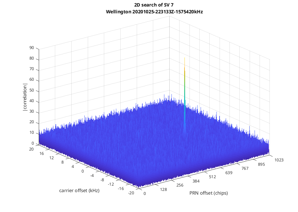 2D search for SV7 in IQ recording
You can see the signal is incredibly peaky so without a brute force search like this it would be a very difficult signal to find indeed. Though this figure is pretty it has so many points that it makes my computer sluggish to work with so this will be the only time I produce one of these pesky plots. The larger the number of PRNs in the PRN block the lower the noise floor compared to the peak as long as you don’t cross a navigation data bit that changes; which may happen every 20 PRNs.
Matlab classes
If we carry on like this we are going to have a huge totally unreadable Matlab script; so we’ll have to move a lot of the code into other files. Even then it’s going to be messy. I am mainly going to write classes but I’ll write the occasional function script when appropriate. All my classes will have the same kind of template and just one or two functions in them to do the hard work. Partly my use of classes is to have a place to store variables for a given functional block.
So here is the class that is responsible for finding coarse carrier frequency and PRN offset using the 2D search just described…
classdef search_2d_for_prn_class < handle
    %search for prn in chip phase and cariier frequency
    %

    properties
        prn_block;%consists of many prns
        prn_len;%length of 1 prn in the prn_block
        max_freq_offset_to_try_in_hz;
        Fs;
    end

    properties (GetAccess = public , SetAccess = private)
        frequency_offset_in_hz;
        chip_offset_in_samples;
        correlation;
    end

    properties (GetAccess = private , SetAccess = private)
        cB;
    end

    methods

        function Reset(obj)
            obj.max_freq_offset_to_try_in_hz=10000;
            obj.Fs=8000000;
            obj.prn_len=8000;
            obj.prn_block=zeros(40000,1);
            obj.frequency_offset_in_hz=0;
            obj.chip_offset_in_samples=0;
            obj.correlation=1;
        end

        function obj = search_2d_for_prn_class()
            obj.Reset();
        end

        function set.prn_block(obj,value)
            obj.prn_block=value;
            %precomputing for the correlation, basically this is what we are
            %doing cor=ifft(fft(signal).*conj(fft(prn))) but the size of a might be
            %different so we get frational frequency offsets
            obj.cB=conj(fft(obj.prn_block));
        end

        function obj = search(obj,signal)

            prn_block_len_in_samples=numel(obj.prn_block);

            assert(prn_block_len_in_samples==numel(signal),'signal and prn block should be same lengths');
            assert(mod(prn_block_len_in_samples,obj.prn_len)==0,'number of prns in prn_block needs to be a whole number');

            %calc shift in freq domain for freq offset
            hz_per_bin=obj.Fs/prn_block_len_in_samples;
            max_freq_shift_to_try=ceil(obj.max_freq_offset_to_try_in_hz/hz_per_bin);
            assert(max_freq_shift_to_try>=0,'max_freq_shift_to_try should not be negative');

            %precomputing for the correlation, basically this is what we are
            %doing cor=ifft(fft(signal).*conj(fft(prn))) but the size of a might be
            %different so we get frational frequency offsets
            A=fft(signal);

            %something to save the best correlation and the freq offset of it
            maxcorr=0;
            maxcorr_freq_shift=0;
            maxcorr_chip_shift=0;

            %the 2d search itself
            for tmp_freq_shift=-max_freq_shift_to_try:max_freq_shift_to_try
                As=circshift( A, tmp_freq_shift );
                circcorr_xy = ifft(As.*obj.cB);
                [tmp,tmp_chip_shift]=max(abs(circcorr_xy(1:obj.prn_len)));% we dont have to go any further than prn_len_in_samples as the prn repeats after that
                if(tmp>maxcorr)
                    maxcorr=tmp;
                    maxcorr_freq_shift=tmp_freq_shift;
                    maxcorr_chip_shift=tmp_chip_shift;
                end
            end

            %calc best freq, chip offsets, and correlation
            obj.frequency_offset_in_hz=maxcorr_freq_shift*hz_per_bin;
            obj.chip_offset_in_samples=maxcorr_chip_shift;
            obj.correlation=maxcorr/prn_block_len_in_samples;

        end
    end

end
Tracking
Now we have to deal with the trickier issue of tracking using our estimates of carrier frequency and chip offset or PRN offset obtained from the 2D search. For this we have to make sure both the carrier frequency offset and PRN phase offset are not too big such that the correlation doesn’t work; if one fails we have to start the whole 2D search again.
The following figure shows a block diagram of the tracking I’m proposing to use…
I’m not sure how good this tracking will be for calculating position solutions, but currently my main goal just to be able to track the signal and then decode the navigation data; if I do manage to obtain position solutions, well then that’s just gravy.
NCO stands for numerically controlled oscillator. I use the term wave table for them too. The idea of them is you have a table with something like a sine wave in it and step through it with a certain stride to produce a sine wave that can be any frequency you want; a big stride is a high frequency, a small stride a low frequency. For a PRN NCO instead of using sine wave you fill up the table with the PRN and everything else is the same as the sine wave example. So at any instance in an NCO you will have a certain location and a certain stride, this is the same thing as saying will have a phase and a frequency. Phase is with respect to the first entry in the table.
The input signal into the block diagram is complex. When put the input signal through the first mixer the frequency offset of the received signal is reduced with the aim to have its output frequency offset as small as possible but the signal will still unavoidably be spinning slowly. The slowly spinning signal can then be mixed with the PRN to remove the spreading signal transmitted by the satellite. This then goes into a prompt integrate and dump module (I&D) where the dumping is triggered by each zero phase crossing of the PRN NCO for the prompt I&D.
There are two more integrate and dump modules, early and late, which have the slowly spinning signal mixed with an advanced and a retarded output from the PRN NCO as their inputs respectively. For these two integrate and dump modules approximately every 15th PRN causes the modules to dump; these modules don’t monitor the PRN NCO for zero crossings. The output from these integrate and dump modules are used so we can produce a PRN error signal to adjust our PRN NCO such that it matches the incoming signal, which is basically a PRN repeating over and over again.
An integrate and dump module keeps adding its input to an accumulator (this is the integration part) and at some later point in time will output the value in this accumulation will reset it to zero (this is the dump part).
So speed wise there are three sections, one running at 8 MHz one running at 1 kHz and one running at about 67 Hz. The one running at 67 Hz is responsible for updating the PRN NCO. Its error detector (ED) could be all sorts of things but I am going to make it the difference between the absolute values from the integrate and dump modules (chip_tracking_error=(abs(chip_tracking_early)-abs(chip_tracking_late));). The output from this error detector is adjusted by a couple of gains and nudges the frequency offset as well as the phase offset of the PRN NCO.
The carrier tracking is mainly implemented in the 1 kHz section. It is divided into two parts, a PLL (phase locked loop) and a FLL (frequency locked loop). After the prompt integrate and dump module, the signal is put through an AGC. Without the AGC the carrier phase and frequency detectors won’t work properly. To stop the slow spinning the output from the AGC is fed into a PLL, consisting of a mixer, a 0 Hz NCO, phase detector (PD) and a gain block. The PLL’s PD is carrier_phase_error_signal=sign(real(point_bit))*imag(point_bit);.
As the navigation data is mixed with the PRN in the satellite the PRN will periodically flip between being inverted and not inverted. The FLL uses the same input as the PLL except it also needs to know whether or not the PRN inverted or not. This information is obtained from the output of the PLL by taking the real component of and making a hard decision whether or not it is greater or less than zero. This is then mixed in with the same signal PLL uses. This new mixed-signal is slowly spinning but has no navigation data so is just the point slowly spinning. The frequency detector (FD) monitors the difference between consecutive points to produce an error signal proportional to the frequency offset (carrier_freq_error_signal=imag(point)*real(point_last)-imag(point_last)*real(point);). This error signal is put through a gain block and fed into the carrier frequency NCO.
Phew! I hope that kinda makes sense and I’ve converted my Matlab code into a block diagram correctly. It’s Matlab where everything really needs to be done in blocks else it’s just too slow so that greatly complicates this kind of thing. From the block diagram above you don’t see where things are done in blocks, it just looks like I’m performing one sample at a time which is how I would implement most of it in C++. So it’s a little misleading but hopefully you get the idea of the components I’m putting together. Looking at it now there are some things I might change but it’s good enough to get started. Now, let’s run through the Matlab classes that make up this block diagram.
PRN NCO class
Because of the block nature of Matlab this is one of the most confusing classes; it looks like this…
classdef prn_block_nco_class < handle
    %prn nco that takes a block at a time of M prns
    %

    properties
        phase;     %current phase in chips for this sample (after calling "next", phase will be for the last sample in the vector)
        frequency; %in chips per ms
        block_len; %block length in samples
        Fs;        %sample rate in Hz
        sv;        %sv number
    end

    properties (GetAccess = public , SetAccess = private)
        prn;
        block;

        zero_phase_crossing_index;
        zero_phase_crossing_fractional;
    end

    properties (GetAccess = private , SetAccess = private)
        last_phase;
        last_sample_crossing_item;
    end

    properties (Constant)
        prn_len=1023;
    end

    methods

        function Reset(obj)
            obj.sv=1;
            obj.Fs=8000000;
            obj.phase=0;
            obj.last_phase=0;
            obj.zero_phase_crossing_index=[];
            obj.last_sample_crossing_item=-inf;
            obj.frequency=obj.prn_len;
            obj.block_len=(obj.Fs/1000)*obj.prn_len/obj.frequency;%1000 as freq is in ms not s
        end

        function obj = prn_block_nco_class()
            obj.Reset();
        end

        function set.sv(obj,value)
            obj.sv=value;
            obj.prn=2*(cacode(value)'-0.5);
        end

        function prn_block=next(obj)

            x=(obj.frequency)*obj.block_len/(obj.Fs/1000);
            a=linspace(0,x,obj.block_len+1)+obj.phase;
            prn_block=obj.prn(mod(floor(a(1:obj.block_len)),obj.prn_len)+1);%1023 here is prn len
            obj.block=prn_block;

            %for prn crossing
            block_phase=mod((a(1:obj.block_len)),obj.prn_len);
            block_phase_delta=block_phase-[obj.last_phase,block_phase(1:end-1)];
            obj.last_phase=block_phase(end);

            obj.zero_phase_crossing_fractional=[];
            obj.zero_phase_crossing_index=[];
            index=find(block_phase_delta<(-obj.prn_len/2));%only interested in +ve crossings of the prn
            for k=1:numel(index)
                delta_samples=index(k)-obj.last_sample_crossing_item;
                obj.last_sample_crossing_item=index(k);
                if(delta_samples>(((obj.Fs/1000)*obj.prn_len/obj.frequency)/2))
%                     fprintf('crossing detected at sample %d of this vector\n',index(k));
                    obj.zero_phase_crossing_index(end+1)=index(k);%integer crossing point
                    obj.zero_phase_crossing_fractional(end+1)=index(k)-block_phase(index(k))/((obj.frequency)/(obj.Fs/1000));%for crossing point with fractional res
                end
            end
            if(numel(index)>0)
                obj.last_sample_crossing_item=index(end)-obj.block_len;
            end

            %points to next sample as phase
            %no mod. if you want mod then do that elsewhere
            obj.phase=a(end);

        end
    end

end
Yeah it’s not easy to understand. It consists of two parts. The first part figures out all the phases to place in the vector a, using this vector it figures out what should go into the PRN block to be returned, and updates the phase for the next block. The second part deals with detecting when zero crossings of the phase happens and creates two vectors zero_phase_crossing_index and zero_phase_crossing_fractional that point to where in the block the zero crossings occur.
Note that its phase upon finishing does not mod 1023. Internally it will still calculate zero crossings of PRNs even though its phase will continue to increase. It’s up to the instance owner of this class to do any modding of multiples of 1023. This set up is so when the first PRN of the second arrives, mod 1023 can be done on the phase then. What I mean by this is imagine the time has just transitioned from 11:15AM to 11:16AM and you are less than a millisecond after 11:16AM then mod the phase by1023 then. This means the phase will represent the fractional part of any second in the uncorrected satellites transmit time. I’ll explain more about this later.
Integrate and dump class
This one’s pretty simple and isn’t that critical if you’re out a sample here or there…
classdef integrate_and_dump_class < handle
%intgrate and dump a signal
%
properties
dumps;
dumps_count;
end
properties (GetAccess = private , SetAccess = private)
running_integration_sum;
running_integration_count;
end
methods
function Reset(obj)
obj.running_integration_sum=0;
obj.running_integration_count=0;
obj.dumps=[];
obj.dumps_count=[];
end
function obj = integrate_and_dump_class()
obj.Reset();
end
function obj = next(obj,signal,dump_index)
obj.dumps=[];
obj.dumps_count=[];
last_sample=1;
for k=1:numel(dump_index)
start_sample=dump_index(k);
this_count=start_sample-1-last_sample+1;
this_sum=sum(signal(last_sample:start_sample-1));
obj.running_integration_count=obj.running_integration_count+this_count;
obj.running_integration_sum=obj.running_integration_sum+this_sum;
%dump the sums for the user
obj.dumps(end+1)=obj.running_integration_sum;
obj.dumps_count(end+1)=obj.running_integration_count;
last_sample=start_sample;
obj.running_integration_sum=0;
obj.running_integration_count=0;
end
%save partial sums for later
this_count=numel(signal)-last_sample+1;
this_sum=sum(signal(last_sample:end));
obj.running_integration_count=obj.running_integration_count+this_count;
obj.running_integration_sum=obj.running_integration_sum+this_sum;
end
end
end
As an input it takes a signal as well as an index as to when to dump the accumulator. For the prompt integration dump module, the dump index is obtained from the PRN NCO zero crossings.
This class is not used for early or late integrate and dump modules.
AGC class
This one I used a sample by sample implementation as it’s only running at 1 kHz so is extremely straightforward…
classdef agc_class < handle
    %agc for a signal of complex points
    %

    properties
        agc_val;
        alpha;
        signal_out;
    end

    methods
        function Reset(obj)
            obj.agc_val=1;
            obj.alpha=0.1;
            obj.signal_out=[];
        end

        function obj = agc_class()
            obj.Reset();
        end

        function obj = update(obj,signal_in)

            obj.signal_out=signal_in;
            %update agc
            for k=1:numel(signal_in)
                if(isnan(signal_in(k)))
                    obj.signal_out(k)=1;
                    continue;
                end
                x=abs(signal_in(k));
                if(obj.agc_val<0.00000001)
                    obj.agc_val=0.00000001;
                end
                if(obj.agc_val>1000000000)
                    obj.agc_val=1000000000;
                end
                obj.agc_val=1/((1/obj.agc_val)*(1-obj.alpha)+obj.alpha*x);

                %scale points using agc_val
                obj.signal_out(k)=signal_in(k).*obj.agc_val;

            end
        end
    end

end
Carrier tracking class
This one combines the PLL with most of the FLL. This class again lives in the 1 kHz section. Therefore it doesn’t contain the carrier NCO nor does it update its frequency, that is done 67 Hz section which happens once every block. It does however contain the 0Hz NCO but this is simply the line point_bit=point*exp(-1i*2*pi*obj.phase_offset);…
classdef carrier_point_bpsk_phase_tracker_class < handle
    %removes rotation of bpsk points and estimates frequency offset
    %

    properties
        frequency_offset;
        phase_offset;

        %for phase error gain
        phase_error_gain;
    end

    properties (GetAccess = public , SetAccess = private)
        carrier_phase_error_signal;
    end

    properties (GetAccess = private , SetAccess = private)
        point_last;
        fll_b;
        fll_a;
        zi;
    end

    properties (Constant)
        frequency=1000;%because 1000 prns a second

        %for carrier FLL loop filter
        lpf_3db_freq=10;%in hz
        lpf_order=2;%2 should do

    end

    methods
        function Reset(obj)
            obj.frequency_offset=0;
            obj.phase_offset=0;
            obj.carrier_phase_error_signal=0;
            obj.point_last=0;
            obj.phase_error_gain=0.18;

            %carrier FLL loop filter
            [obj.fll_b,obj.fll_a] = butter(obj.lpf_order,obj.lpf_3db_freq/(obj.frequency/2));
            obj.zi=zeros(obj.lpf_order,1);

        end

        function obj = carrier_point_bpsk_phase_tracker_class()
            obj.Reset();
        end

        function points=update(obj,points)
            carrier_freq_error_signal_sum=0;
            for k=1:numel(points)
                point=points(k);

                %remove current phase offset
                point_bit=point*exp(-1i*2*pi*obj.phase_offset);
                %calc phase error and update phase_offset
                obj.carrier_phase_error_signal=sign(real(point_bit))*imag(point_bit);
                obj.phase_offset=obj.phase_offset+obj.phase_error_gain*obj.carrier_phase_error_signal;

                %remove nav signal from point before phase offset removed. needed
                %for frequency tracking algo
                if(real(point_bit)<0)
                    point=point*exp(1i*pi);
                end

                %calc frequency offset
                carrier_freq_error_signal=imag(point)*real(obj.point_last)-imag(obj.point_last)*real(point);%approx angle between 2 points. delta rad per delta time(1/1000)
                carrier_freq_error_signal=obj.frequency*carrier_freq_error_signal/(2*pi);%convert into Hz
                [carrier_freq_error_signal,obj.zi]=filter(obj.fll_b,obj.fll_a,carrier_freq_error_signal,obj.zi);
                obj.point_last=point;
                carrier_freq_error_signal_sum=carrier_freq_error_signal_sum+carrier_freq_error_signal;

                %return the corrected point
                points(k)=point_bit;
            end
            obj.frequency_offset=carrier_freq_error_signal_sum/numel(points);
        end

    end

end
This is the final class used for the carrier and PRN tracking, the rest is done in the main unit.
AGC output
Nothing much can be seen along the signal path until we get to the AGC. The following figure shows the output from the AGC for satellite vehicle number seven…
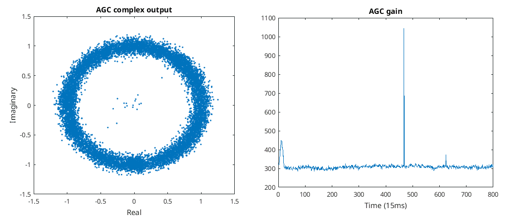 Output of the AGC
The output from the AGC is unusual compared to the other modulation schemes I’ve dealt with. Because we are correlating over each PRN and are making sure not to correlate over PRN NCO zero phase crossings, the output looks like a circle with nothing in the center. As the figure on the left is a circle this means the BPSK from the satellite navigation data is slowly rotating.
The figure on the right is the gain that is being applied to the signal that goes into the AGC. When the PRN signal is well correlated the AGC gain should decrease while when the PRN signal is not well correlated the AGC signal should increase. At the very beginning you see a small blip when the AGC goes up to about 450 and then drops down to about 300; this is caused due to the PRN NCO better estimating the phase and frequency of the incoming PRN signal. More interestingly at around seven seconds and again nine seconds we see two more blips with very sharp peaks. It’s pretty clear to me what this is. These two peaks are almost certainly due to USB packets being dropped between the SDR play and the computer. This is always a problem when capturing data on general purpose computers, I’ve had this issue a lot with soundcards the past. It takes only the dropping of one tiny little packet to totally mess a perfectly good link. I do wish people would be more careful when designing software and hardware to avoid this issue. Anyway that’s what we have to face with in this 12 second recording.
Output of the PLL (out)
The PLL takes the output from the AGC and stops it spinning; this is its output…
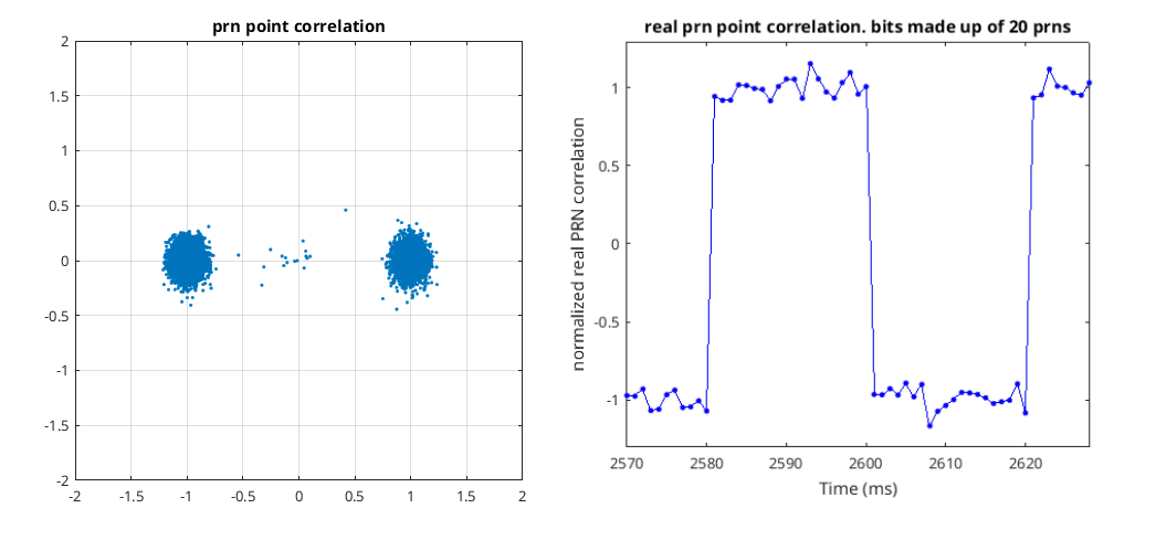 Output from PLL (out)
What’s interesting here is it already looks like BPSK, yet we haven’t done any symbol timing in the traditional sense by using an algorithm like the gardener algorithm. Magically points seem to cross instantaneously between +1 to -1 without ever having to slowly meander through the middle.
In the right figure we see just the real component. You can see that there are exactly 20 points once it goes to +1. Then, when it goes back to -1 there are again exactly 20 points. In fact there are always exactly 20 points per bit as 20 PRN’s makeup one bit and bit transitions always happen at the beginning of a PRN. Therefore we can number these PRN points from 0 to 19 inclusive. The 0th PRN is important as seconds are always aligned to them, i.e. every 50th 0 PRN happens on the second; of course at the moment we don’t know which one. Anyway I’m getting ahead of myself; firstly I’ll finish off looking through the tracking stuff.
Carrier error signals
The carrier error signals consist of the phase and frequency error signals. These drive two separate NCOs. The frequency error signal drives the frequency component of the NCO marked as “f NCO” in the tracking diagram, while the phase error signal drives the phase component of the NCO marked as “0Hz NCO”. The frequency error signal comes out of a low-pass filter (marked as “LPF” in the diagram), while phase error signal comes out of the phase detector (marked as “PD” in the diagram). The units are Hertz and radians respectively. The following figures shows the output of these error signals…
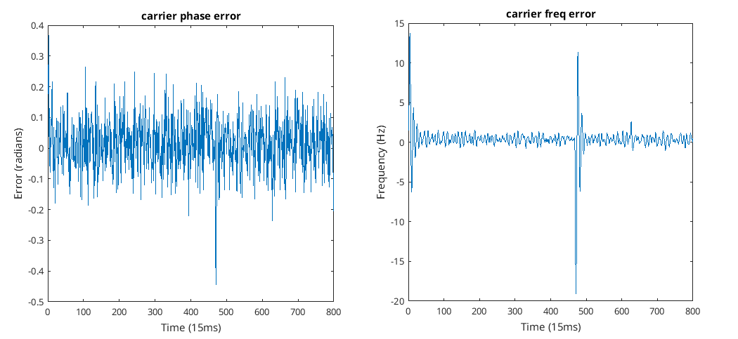 Carrier error
So you can see both are around zero with a bit of noise. That is the reason why I have gain blocks to reduce the level before adjusting the NCOs with these signals. If the gain is too low tracking fails because it doesn’t have enough agility, while if the gain set is too high it will madly oscillate or be unstable; either case tracking fails. The way I set these things is by initially having no frequency gain, increase the phase gain until the signal locks, then increase the frequency gain such that I see the phase error signal around zero, i.e. no phase error signal bias.
While we are here we might as well look at the frequency of the “f NCO”…
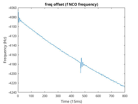 Carrier frequency offset
Again like in all these other plots you see the pesky USB buffer drop at around seven seconds which seems to be the worst of the two. This figure seems to looks okay. As satellites move toward or away from you their frequency changes due to the Doppler Effect. This effect is the same one that causes emergency services sirens on vehicles to sound different when the vehicle is moving towards you or away from you. However I don’t know how much of the frequency shift that can be seen in the previous figure is due to the instability of the oscillator inside the SDR play. Darren from the UK is kindly sending me an updated version of the SDR play called RSP1A which has a temperature compensated crystal oscillator and will be interesting to compare the two receivers.
PRN tracking
As the output from the early and late integrate and dump modules are 15 PRNs long we will inevitably sometimes cross navigation data bit transitions. The effect of this will be to reduce the correlation. This is not ideal but as both the early and late integrate and dump modules will suffer similarly, the effect on the PRN error detector called “ED” in the block diagram will reduce its output but hopefully shouldn’t change the sign of the error. The figures below show the output of a prompt integrate and dump module over 15 PRN’s long with the one on the right being a close up view of part of the one on the left…
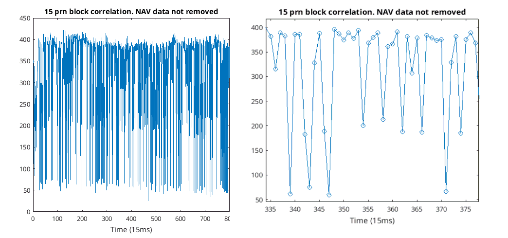 PRN block correlation. Dips are due to bit crossing.
Ideally every correlation should be around 400 in this case, but due to the navigation data bit crossings during the correlation (mixing PRN, integrating and dumping) we sometimes see significant drops in correlation of up to 90%.
The output of the early and late correlations are fed into the PRN error detector (“ED”). The ED is the simplest one you could possibly think of, chip_tracking_error=(abs(chip_tracking_early)-abs(chip_tracking_late));. A plot of this over time can be seen in the following figure…
In this case it took about half a second for it to adjust the frequency and phase of the PRN NCO to good estimates and reduce the PRN tracking error to around zero.
The frequency offset from the nominal 1000 PRN/s for the PRN NCO can be seen in the following two figures where the one on the right is a close up view of the one on the left…
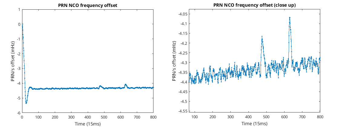 PRN frequency offset
I have seen mention to a PRN NCO tracking loop that uses something called carrier aided tracking. This uses a carrier error signal to adjust the PRN NCO somehow. From my understanding it requires the timing of the ADC in the receiver to be phase linked with the front-end receiver mixer. In addition I think one also might need to know the fractional difference between the ADC sampling frequency and the front-end receiver mixer but I’m not sure. Being phase linked would mean you just require a receiver that uses just one crystal to drive everything and this is probably the case in most receivers including the SDR play. However when I tuned the SDR play to 1575.42MHz I doubt that it’s actually able to tune to exactly that frequency and hence why when I made a recording at that frequency it called it “SDRuno_20201025_223133Z_1575409kHz” meaning it’s about 11 kHz out. Even then I don’t know if that’s exactly the frequency it wanted to tune to. 1575.409/8=196.926125 so is not a simple multiple of 8 MHz. On the satellite 1575.42MHz=15401.023MHz, in other words the carrier frequency is an integer multiple of the chip rate and they are phase linked to the same clock. If I had a receiver that would do a similar thing I could use the carrier frequency offset divided by 1540 to find the PRN chip frequency offset; I believe this is what carrier aiding is. For us things will be a bit different, so let’s plot freq_offset+1540*((prn_nco.frequency-1023)*1000). freq_offset is the carrier offset frequency we are tracking while prn_nco.frequency is the PRN NCO frequency in chips per millisecond so ((prn_nco.frequency-1023)*1000) is the PRN NCO chip frequency offset in Hz. The reason I added these numbers rather than subtracting them is because I mucked up and got the sign of one of the two back to front depending on the way you look at it. I’m not going to change it just now for consistency; it doesn’t really matter that much. Anyway here are the plots the right one being a close-up of the left one…
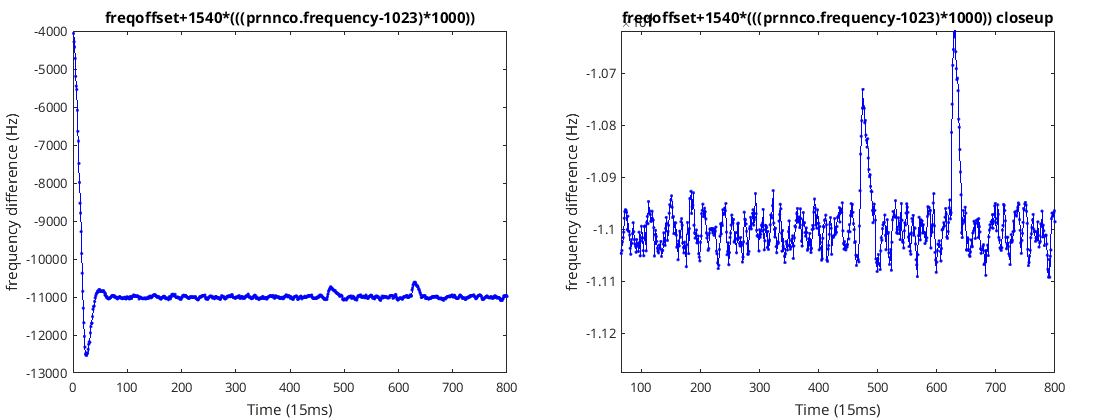 Carrier frequency offset and linear scaled PRN frequency offset
So there are a couple of interesting things about these plots. One is how flat it is, and the other one is that it seems to settle on -11 kHz. It’s very similar to the previous plots the main differences these ones are very flat.
So it looks like we could use carrier aiding, we just have an offset of 11 kHz to deal with. It would mean we would either have to allow the user to enter the receiver’s front-end offset or calculate this offset first before using it. The reason for doing carrier aiding would be to use the lower noise of the carrier frequency estimation. The only reason for doing it would be to get a better position solution rather than for simply obtaining navigation data.
The initial chip frequency from the satellite is 1023 chips per millisecond . This is mucked up by Doppler and by the time we receive the signal the chip rate is .
As one crystal controls both the front-end mixer and the ADC there must be some real number (probably fractional) such that the carrier frequency offset at the input to the ADC can be written as follows…
The chip rate offset at the input of the ADC is not affected by the front-end mixer so can be written as follows…
Measured frequencies in the digital domain depend on what frequency we believe the ADC to running at and the actual frequency of the ADC. Therefore, we can write these measurements as follows…
Multiplying the measured chip frequency offset in the digital domain by 1540…
While the measured carrier offset in the digital domain is…
Taking the difference we obtain the frequency difference we measure in the digital domain…
Where is the receiver’s frequency tuning offset to the nominal 1575.42 MHz. So we don’t quite measure it as a constant in the digital domain and it depends a tiny bit on the ADC’s sample rate. If we assume the SDR play has a crystal with a 20 ppm and we know is about 11 kHz we expect an error of around 0.2 Hz which I don’t think is going to be that significant. It would be nice to know what m is, my guess is it is a fractional number. To know what it actually was you have to know how the SDR play generated its timing from its crystal. It’s interesting that we can use these satellites to measure the frequency tuning offset of the SDR play. Anyway we have shown that indeed there is a constant relationship between 1540 times the measured chip rate offset and that of the measured carrier offset; so that’s why it works.
With this carrier aiding we can rewrite the tracking block diagram to the following…
All we have done is remove the frequency updates to the PRN NCO from the ED and instead are controlling the PRN NCO via a linear function whose input is the carrier NCO frequency.
Using the previous equations we can write the following formula that describes the received chip rate in terms of the carrier frequency offset and tuning frequency offset.
This is our linear function with respect to the carrier frequency offset. Carrier frequency offset is the carrier NCO frequency block element, while the tuning offset is the one measured which is about -11 kHz. The output of this function is the PRN NCO frequency in Hertz.
For my current implementation I have some of the signs mixed up and the PRN NCO frequency is in terms of MHz so that changes things just a little in my implementation. The following shows the code that updates both the PRN NCO. Carrier aiding can either be enabled or disabled.
%use EL chip error to adjust chip phase. frequency uses either
%carrier aiding or EL chip error
prn_nco.phase=prn_nco.phase+chip_tracking_error*chip_tracking_error_phase_gain;
%if carrier aiding
if(use_carrier_aiding)
    prn_nco.frequency=(tuner_frequency_offset_for_carrier_aiding-freq_offset)/(1540*1000)+1023;
else
prn_nco.frequency=prn_nco.frequency+chip_tracking_error*chip_tracking_error_freq_gain;
end
The following two figures show output from the PRN error detector (ED) without and with carrier aiding…
You can see in both cases the error is around about zero, this shows that we have made carrier aiding correctly. You can see with carrier aiding the error goes to zero much more quickly. This is because the coarse acquisition has given the carrier NCO an initial frequency guess which in turn gives the PRN NCO and initial frequency guess, so that’s nice.
In the following two figures I have applied a high-pass filter to the PRN NCO frequency offset for both without carrier aiding and with carrier aiding; both figures have the same scale…
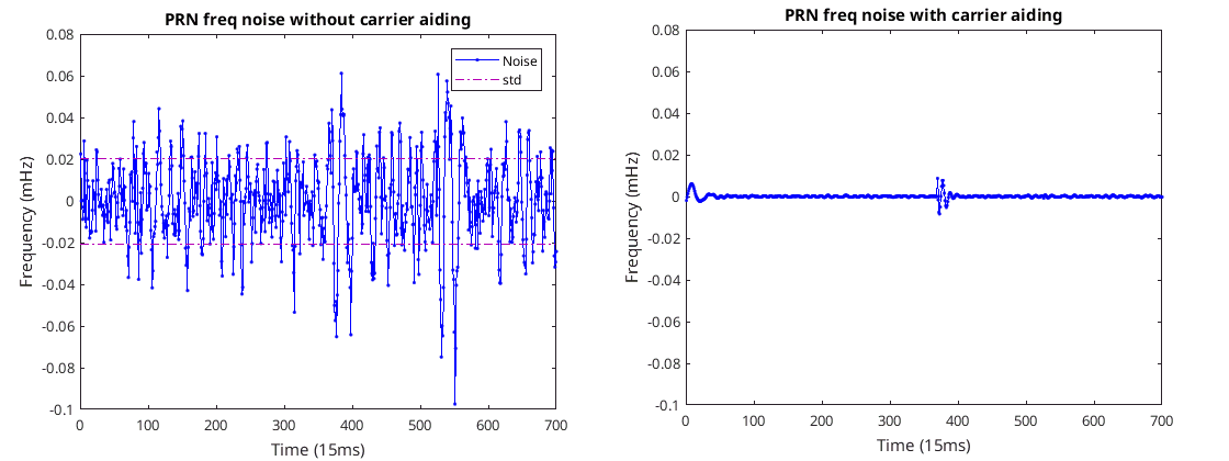 PRN frequency noise with and without carrier aiding
Doing this high-pass filtering you get to see the noise of the signal. Having low noise is good for accuracy. Without carrier aiding there is about 0.02 mHz standard deviation, while with carrier aiding we get about 0.001 mHz so that’s an order of magnitude better.
I’m definitely going to use this carrier aiding and unless otherwise mentioned I will use this for the rest of this document.
What satellites are detectable?
While we can use a satellite tracking programs to figure out what satellites are in view that doesn’t necessarily mean we can detect their signals. So let’s run a 2D search on each of the 32 PRNs that we know about see correlation is like for each of the satellites. Most likely at least 50% of the satellites we won’t be detectable as they will be below the horizon, so we can use the 16 weakest correlations to figure out the noise floor value and standard deviation. Anything that is significantly higher than the noise floor we can regard as being a signal. To get good sensitivity for this figuring out what satellites are detectable I am going to use a PRN block of 20 PRNs and even then I’m going to sum four these together. Here is the code used figure out what satellites are detectable and get an idea of how strong signals are to one another…
% find what svs we can see

%number of wanted prns to correlate over
prns_per_correlation=20;

samples_per_prn=Fs/prns_per_second;
samples_per_correlation=samples_per_prn*prns_per_correlation;

% prn nco
prn_nco=prn_block_nco_class();
prn_nco.block_len=samples_per_correlation;
prn_nco.Fs=Fs;
prn_nco.sv=1;
prn_nco.phase=0;
prn_nco.frequency=1023;
%

% 2d search
search_2d=search_2d_for_prn_class();
search_2d.Fs=Fs;
search_2d.max_freq_offset_to_try_in_hz=20000;
search_2d.prn_block=prn_nco.next();
search_2d.prn_len=samples_per_prn;
%

svs_corr=zeros(32,1);
for sv=1:32
    found_sv=false;

    %set sv number to try
    prn_nco.sv=sv;
    search_2d.prn_block=prn_nco.next();

    %look through 4 blocks and take max.
    %we know we can get a big
    %reduction in corr so this will help
    %to avoid that issue.
    abs_corr_sum=0;
    for m=0:3
        %get a block of signal
        a_org=y(samples_per_correlation*m+1:samples_per_correlation*(m+1));

        %search for signal changing the prn phase given a nominal 1023
        %chips/s chip rate and also the carrier freq
        search_2d.search(a_org);

        abs_corr_sum=abs_corr_sum+search_2d.correlation;
    end

    %print and save corr to array
    fprintf("sv=%d corr=%f\n",sv,abs_corr_sum);
    svs_corr(sv)=abs_corr_sum;
end

%sort corr in decending order
[svs_corr_sorted,svs_sorted]=sort(svs_corr,'descend');
%we can only see 50% of sv max on earth so use the weakest svs as noise ref
%and remove this from our result. anything above we assume to be a signal
svs_corr_sorted=svs_corr_sorted-max(svs_corr_sorted(17:end))-3*std(svs_corr_sorted(17:end));
svs_corr_sorted=svs_corr_sorted./svs_corr_sorted(1);
%display the results
plot(svs_sorted,svs_corr_sorted,'o')
ylim([0 svs_corr_sorted(1)+3*std(svs_corr_sorted(17:end))./svs_corr_sorted(1)]);
xlim([0 33]);
%make the a list of detectable svs
svs=svs_sorted(svs_corr_sorted>0);
I used prn_block_nco_class as it was an easy way to create concatenated PRN which is required for the 2D search class.
This code is very slow to run and takes quite a few minutes to complete. Normally you wouldn’t brute force search every single satellite and would rather find one satellite, get the approximate time and almanac from that satellite which would tell you where approximately all the satellites are. You would guess your extremely approximate location as either the last position solution you calculated (for me New Zealand) or failing that just take your approximate location as being directly underneath the current satellite your tracking. Then you only search for the satellites that are in view. Anyway, that’s not what I’m going to do here mainly because that’s more complicated and requires more navigation data than I can probably get from my 19 seconds recording.
The plot that this code produces of the correlations of the satellites can be seen in the following figure…
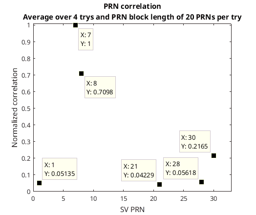 Relative corellation for detectable svs
Anything below zero I’m regarding as something that I can’t detect. SVs 7 and 8 are by far the strongest signals. When we try going for the weaker signals 1,21,28 and 30 we will see that even SV 30 is pretty weak.
According to Obitron the satellites visible were 1,7,8,21,28,30,4,9,11,13,16, and 27. Every single one I detected was in the list so that’s good but I only managed to detect half of the 12 that were supposedly visible.
Anyway, this saves a lot of effort because I only have to attempt to track the first six satellites at most.
Bit synchronization
The data that is sent by the satellites is called navigation data and is sent at 50 bits per second by flipping the PRN signal so instead of sending say 01100 the satellite would send 10011. It contains the time, almanac, ephemerides, health of the satellite etc.
As I mentioned earlier there are always exactly 20 PRNs per bit and we can number each of these PRNs from 0 to 19. The very first PRN after a bit transition is numbered zero. So we need something to figure out which is the first PRN. My idea for this was to take the output from the tracking block diagram I have already described and upon every new output from this block place it into a matrix of N rows by 20 columns in a scanned left to right top to bottom manor. As we know transitions happen every 20 PRNs, if we have enough rows we should see only one column where the value flips. Here are two diagrams to explain what I mean more clearly…
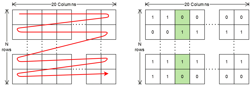 How to find which PRN is the first in a bit. i.e. where is the PRN with sequence number zero.
The one on the left shows how the matrix is filled with the output data from the tracking block. The one on the right shows the data in the matrix. You can see that only between the second and third columns may a value change. Technically here I have taken the real output of the tracking loop and put it through the Heaviside function such that negative numbers are mapped to zero while positive numbers are mapped to one. So in this example whenever we are filling the matrix and the column happens to be the third column, then we currently have in the first PRN.
I made a class to take the output from the tracking block and label each output 0 to 19 using this matrix bit synchronization algorithm. In addition the class performs an integration and dump of the incoming data such that the dumping is performed after all 20 PRN have been summed. This integration of all 20 PRNs creates an output of 50 bits per second and is our navigation data. The following figure shows a block diagram this class…
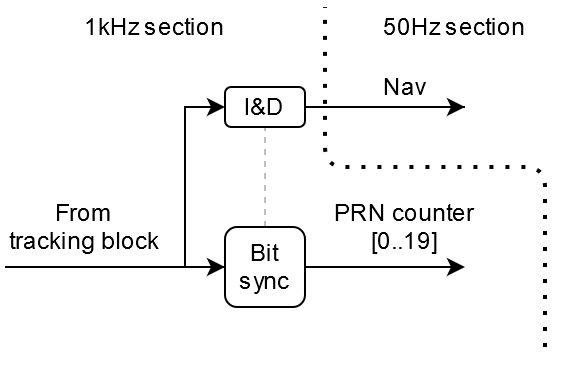 Bit syncronization block.
The class itself is as follows…
classdef bit_sync_class < handle
    %uses 1khz bpsk points to form 50Hz nav data points and prn index for
    %each 1khz bpsk point
    %

    properties
        bit_sync_matrix_row_size;%number of bits to look over for bit/symbol timing

        bit_points;%nav bits (1 is made up of 20 prn points) only valid when prn_number==0.
        prn_numbers;%prn number (0..19 for each prn point)
    end

    properties (GetAccess = public , SetAccess = private)
        bit_sync_matrix;
        bit_sync_matrix_row;
        bit_sync_matrix_col;
        bit_sync_matrix_row_start;
        bit_ave;
    end

    properties  (Constant)
        bit_sync_matrix_col_size=20;%one bit is 20 points in CA gps
    end

    methods

        function set.bit_sync_matrix_row_size(obj,value)
            obj.bit_sync_matrix_row_size=value;
            obj.bit_sync_matrix=zeros(obj.bit_sync_matrix_row_size,obj.bit_sync_matrix_col_size);
        end

        function Reset(obj)
            obj.bit_sync_matrix_row_size=25;
            obj.bit_sync_matrix_row=1;
            obj.bit_sync_matrix_col=1;
            obj.bit_sync_matrix_row_start=0;
            obj.bit_ave=0;
        end

        function obj = bit_sync_class()
            obj.Reset();
        end

        function got_bit=bit_sync_update(obj,points)
            got_bit=false;
            obj.bit_points=nan.*zeros(numel(points),1);
            obj.prn_numbers=zeros(numel(points),1);
            for n=1:numel(points)
                point=points(n);

                %put point into bit sync matrix
                obj.bit_sync_matrix_col=mod(obj.bit_sync_matrix_col,obj.bit_sync_matrix_col_size)+1;
                if(obj.bit_sync_matrix_col==1)
                    obj.bit_sync_matrix_row=mod(obj.bit_sync_matrix_row,obj.bit_sync_matrix_row_size)+1;
                end
                obj.bit_sync_matrix(obj.bit_sync_matrix_row,obj.bit_sync_matrix_col)=heaviside(real(point));

                %find col with most bit transitions
                val_max=0;
                val_max_k_next=1;
                for k=1:obj.bit_sync_matrix_col_size
                    k_next=mod(k,obj.bit_sync_matrix_col_size)+1;
                    if(k_next==1)
                        val=sum(bitxor(obj.bit_sync_matrix(1:end-1,k),obj.bit_sync_matrix(2:end,k_next)));
                    else
                        val=sum(bitxor(obj.bit_sync_matrix(:,k),obj.bit_sync_matrix(:,k_next)));
                    end
                    if(val>val_max)
                        val_max=val;
                        val_max_k_next=k_next;
                    end
                end
                if(obj.bit_sync_matrix_row_start~=val_max_k_next)
                    fprintf('bit sync change was %d now %d\n',obj.bit_sync_matrix_row_start,val_max_k_next);
                end
                obj.bit_sync_matrix_row_start=val_max_k_next;

                %when point of start of bit arrives
                if(obj.bit_sync_matrix_row_start==obj.bit_sync_matrix_col)
                    obj.bit_ave=obj.bit_ave./obj.bit_sync_matrix_col_size;

                    %add bit to return. we probably will only get one bit
                    %at most per call but anyway.
                    got_bit=true;
                    obj.bit_points(n)=obj.bit_ave;

                    obj.bit_ave=0;
                end
                obj.bit_ave=obj.bit_ave+point;

                %add return of what prn number this is 0..19
                obj.prn_numbers(n)=mod(obj.bit_sync_matrix_col-obj.bit_sync_matrix_row_start,obj.bit_sync_matrix_col_size);

            end
        end
    end

end
The reason for using this matrix technique rather than simply assuming that any transition over zero signifies the first PRN, is to work better at lower SNR. For SV 7 it’s not really an issue as the signal is so strong but by the time we start having to deal with SV 28 it’s a must. The following figure shows the real output from the tracking loop for PRN 7 as well as red dots on every output that is considered the first PRN using this matrix technique…
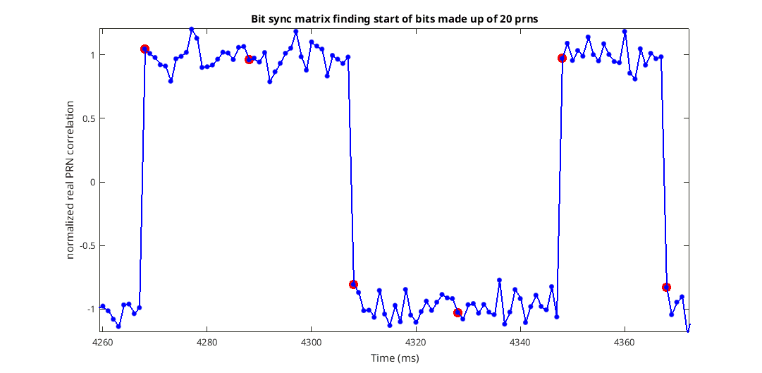 Bit syncronization algorythm applied to signal.
The following two figures show the output from the tracking block and the navigation data output for PRN 28…
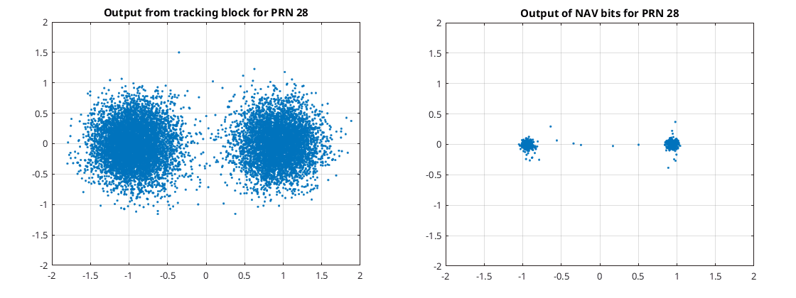 Before and after bit syncronization block
As can be seen there is a significant signal improvement when averaging over 20 points to produce one.
Navigation data overview
Now we finally have navigation data we now need to make a decoder for it. For this we have to wade through the specification documentation. It seems it can be found at USCG GPS technical references. There are about 50 documents on this page; I believe we need the one called “IS-GPS-200 Navstar GPS Space Segment/Navigation User Interfaces”. Of that I guess I will take the 14th of May 2020 edition (IS_GPS_200L.pdf) at 228 pages. Another website where all the documentation can be found is gps.gov. From this documentation we see that there are things called subframes consisting of 10 words and what is transmitted is one subframe transmitted after another where the first word is called TLM, the second word is called HOW, while the last eight words vary and can be thought of as the payload (see “20.3.2 Message Structure”)…
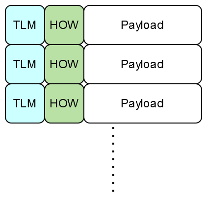 Subframes are concatinated and start with TLM and HOW words
Parity checking is done on each word and consists of 6 bits appended to 24 bits of useful word data.
The TLM word (see “20.3.3.1 Telemetry Word”) consists of a preamble 0x8B, a telemetry message whatever that is, integrity status flag, a reserved bit, and the six bits of parity. The HOW word (see “20.3.3.2 Handover Word (HOW)”) consists of a time of week message, an alert flag, an anti-spoof flag, subframe ID (there are five subframe IDs), 2 bits called t that are set such that the last two bits of the parity are zero, and the parity itself…
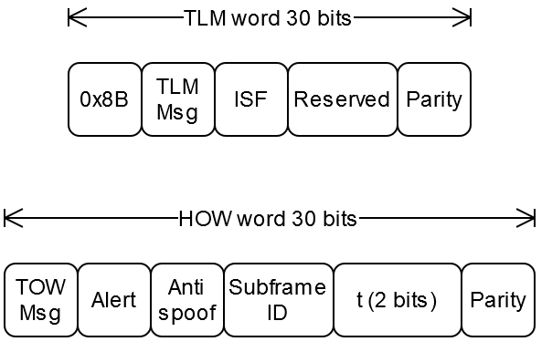 TLM and HOW word formats
The TOW message is the one I’m interested in as it tells you the time at the very beginning of the next subframe in seconds since the week started which is defined as midnight Saturday UTC ish for some bizarre reason. I say ish because it’s GPS time which doesn’t do leap seconds and is 18 seconds ahead of UTC as of writing. The next subframe that TOW refers to is the start of first chip of the first PRN of the first bit of that subframe.
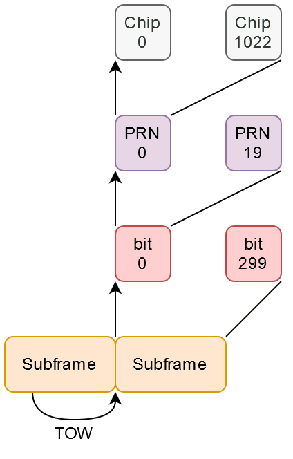 How subframes are aligned all the way to chips
Therefore the TOW allows you to label each chip in a week uniquely, all ish of them, with the transmission time that the satellite sent them at according to its clock.
However, first we need something to find word alignment and to calculate the parity to make sure that the words are correct. Let’s start with the parity check.
Parity check
The parity check they use is rather strange…
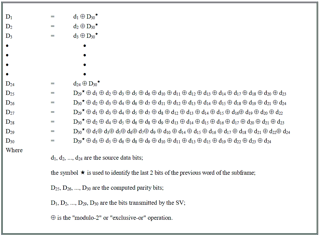 Word parity check; weird
As can be seen the last parity bits D30* and D29* from the previous word effect the current word. So this means when computing the parity check we need to look at the last two parity bits from the previous word which means we have to supply the parity check function with 32 bits rather than 30 bits.
The neat thing about this parity check is that it doesn’t matter if the signal is inverted or not, it has no BPSK phase ambiguity. This is because every row in the equations are multiplied exactly once by one of the two previous parity bits. So if the signal is back to front, D30* and D29* are also back to front which makes all our data bits d1 to d24 the right way round again.
So the idea is to take a 32 bit vector [D29*,D30*,D1,..,D30], xor D1 to D30 by D30* to get d1 to d24, create a parity check matrix and multiply that by [D29*,D30*,d1,...,d24], sum up the resulting vector and if equal to zero the parity check passes. All this is done mod2, Galois field F2 or whatever you want to call it. I have put the following function together to implement this, it returns both whether or not the parity check passes and also the source data d1 to d24 which we want…
function [ ok,word ] = paritycheck( bits )
%paritycheck checks gps nav data parity
% ok true if ok
% bits 32 input bits where the first 2 bits are from the previous word
% word the output word inverted if needed

%check is a 32 bit 0,1 vector
assert(((size(bits,1)==32)&&(size(bits,2)==1))||((size(bits,2)==32)&&(size(bits,1)==1)),'needs a 32 bit vector');
tmp=sort(unique(bits));
if (numel(tmp)==1)
    assert(((tmp(1)==0)||(tmp(1)==1)),'needs to be a binary vector or 0s and 1s');
else
    assert((tmp(1)==0)&&(tmp(2)==1)&&(numel(tmp)==2),'needs to be a binary vector or 0s and 1s');
end

%if D30* then flip data bits
if(bits(2)==1)
    bits(3:26)=1-bits(3:26);
end

%parity check matrix

%D29*,D30*,d1,...,d24,D25,..,D30

PRow1 = [1,0,1,1,1,0,1,1,0,0,0,1,1,1,1,1,0,0,1,1,0,1,0,0,1,0, 1,0,0,0,0,0];
PRow2 = [0,1,0,1,1,1,0,1,1,0,0,0,1,1,1,1,1,0,0,1,1,0,1,0,0,1, 0,1,0,0,0,0];
PRow3 = [1,0,1,0,1,1,1,0,1,1,0,0,0,1,1,1,1,1,0,0,1,1,0,1,0,0, 0,0,1,0,0,0];
PRow4 = [0,1,0,1,0,1,1,1,0,1,1,0,0,0,1,1,1,1,1,0,0,1,1,0,1,0, 0,0,0,1,0,0];
PRow5 = [0,1,1,0,1,0,1,1,1,0,1,1,0,0,0,1,1,1,1,1,0,0,1,1,0,1, 0,0,0,0,1,0];
PRow6 = [1,0,0,0,1,0,1,1,0,1,1,1,1,0,1,0,1,0,0,0,1,0,0,1,1,1, 0,0,0,0,0,1];

PC  = zeros(6,1);
PC(1) = mod(sum(PRow1.*bits),2);
PC(2) = mod(sum(PRow2.*bits),2);
PC(3) = mod(sum(PRow3.*bits),2);
PC(4) = mod(sum(PRow4.*bits),2);
PC(5) = mod(sum(PRow5.*bits),2);
PC(6) = mod(sum(PRow6.*bits),2);

if(sum(PC)==0)
    ok=true;
else
    ok=false;
end

word=bits_to_n_bit_integers(bits(3:26),24,"big");

end

function [ uD10 ] = bits_to_n_bit_integers( A, n,endian)
%bits_to_n_bit_integers
%Turns vector matrix of bits in A into a vector matrix of
%n bits long numbers.
%B is 1 for a bit matrix
%   Detailed explanation goes here

endianset=false;
if(endian=='big')
    A=flip(A);
    endianset=true;
end
if(endian=='little')
    endianset=true;
end

assert(endianset==true,'set either big or small endian');

B = 1;
% get each group of bits in a column of K.
K = cell2mat(arrayfun(@(bit)bitget(A, B+1-bit), 1:B, 'UniformOutput', 0))';
%make sure there is multiple of B
K = K(:);
while ~(mod(numel(K),n) == 0)
    K = [0;K];
end
K = K(:);
% reshape to have them in 8 packs
K = reshape(K, [n, numel(K)/n])';
% get the uint8 vec.
UD = K*(2.^(size(K,2)-1:-1:0))';

uD10=bi2de(K);

end
Word alignment and subframe decoding
The parity check on a per word basis is not the most resilient to false positives. That being the case I am going to determine the word alignment using the TLM and HOW together. I am going to insist that both TLM and HOW parity checks pass, the TLM preamble is 0x8B, and the last two bits of the parity check for the HOW word are both the same. Every bit that comes along I’m going to shuffle across and check if the constraints are met, if they do then I’m going to say that I have obtained word alignment, subframe alignment. I made the following class to do this, it also converts the TOW message into seconds and displays that in a human readable format…
classdef ca_nav_decoder_class < handle
    %decodes c/a nav data
    %

    properties
        tow;
        subframe;
        subframe_bad_word_count;%if not 10 then at least TML and HOW are valid
    end

    properties (GetAccess = private , SetAccess = private)
        bit_sub_frame_buffer;
    end

    properties  (Constant)

    end

    methods

        function Reset(obj)
            obj.bit_sub_frame_buffer=zeros(1,2+10*30);%2 bits for D29 and D30 of last word and 10 words of length 30 for the data
            obj.subframe=zeros(1,10);%to return words
            obj.subframe_bad_word_count=10;
            obj.tow=nan;
        end

        function obj = ca_nav_decoder_class()
            obj.Reset();
        end

        %50Hz points one at a time please
        function update(obj,bit_point)

            obj.subframe_bad_word_count=10;
            obj.tow=nan;

            %shuffle things over and put in the new bit
            obj.bit_sub_frame_buffer=circshift(obj.bit_sub_frame_buffer,-1);
            obj.bit_sub_frame_buffer(end)=heaviside(real(bit_point));

            %see if we have a good TLM and HOW
            [ok,TLM_word]=paritycheck(obj.bit_sub_frame_buffer(1+30*(1-1):32+30*(1-1)));
            TLM_preamble=bitand(bitshift(TLM_word,-16),255);
            if((ok)&&(TLM_preamble==139))%bit alignment with something that looks like the TML preamble
%                                 fprintf('----got TLM =%s ???\n',dec2bin(TLM_word,24));
                [ok,HOW_word]=paritycheck(obj.bit_sub_frame_buffer(1+30*(2-1):32+30*(2-1)));
%                                 fprintf('----got HOW =%s ???\n',dec2bin(HOW_word,24));
                D29D30=sum(obj.bit_sub_frame_buffer(32+30*(2-1)-1:32+30*(2-1)));
                if((ok)&&((D29D30==0)||(D29D30==2)))%for HOW the last 2 parity bits need to both be the same. this sign of them say if the signal is inverted or not. if 1,1 then we have an inverted signal
                    HOW_subframe_ID=bitand(bitshift(HOW_word,-2),7);
                    %yup matlab 2017a doesn't have hex literals
                    %TOW is for next subframe whitch is now as we have
                    %buffered 1 subrame and are on the start of the prn of the
                    %first bit of the next one
                    HOW_TOW=bitand(bitshift(HOW_word,-7),131071)*6;%0x1FFFF
                    obj.tow=HOW_TOW;
                    HOW_TOW_str=datestr(datetime(HOW_TOW,'ConvertFrom','epochtime','Epoch','1980-01-06'),'ddd HH:MM:SS');
                    %                     fprintf('----got TLM and HOW\n');
                    if(D29D30==2)
                        fprintf('signal is inverted\n');
                    end
                    fprintf('----Subframe ID=%d TOW: %s gps\n',HOW_subframe_ID,HOW_TOW_str);
                    fprintf('----%s\n',dec2bin(TLM_word,24));
                    fprintf('----%s\n',dec2bin(HOW_word,24));
                    obj.subframe(1)=TLM_word;
                    obj.subframe(2)=HOW_word;
                    obj.subframe_bad_word_count=0;
                    for word_n=3:10
                        [ok,word]=paritycheck(obj.bit_sub_frame_buffer(1+30*(word_n-1):32+30*(word_n-1)));
                        obj.subframe(word_n)=word;
                        if(ok)
                            fprintf('----%s\n',dec2bin(word,24));
                        else
                            fprintf('----%s bad\n',dec2bin(word,24));
                            obj.subframe_bad_word_count=obj.subframe_bad_word_count+1;
                        end
                    end
                    if(obj.subframe_bad_word_count==0)
                        fprintf('----YAY a good subframe\n');
                    else
                        fprintf("----TLM and HOW look ok but if this is a subframe then there are bad words\n");
                    end
                end
            end
        end

    end

end
If you wanted to be stricter you could insist that all words in the subframe pass the parity check. However as I have some weak signals I’m not going to insist on this. Also I am only interested in decoding TLM and HOW words as the ephemerides can be downloaded from the Internet. Running the first 12 seconds of the navigation data from SV28 into this subframe decoder class I only detected one subframe…
----Subframe ID=5 TOW: Sun 22:32:00 gps
----100010110000000101000100
----000110100110100000110111
----010001000000011100110101
----001110010000101110011100
----111111010101110000000000
----101000010000110010011000 bad
----011000110101101110110110
----100001011111001000101101
----001000010000111111111011
----111011001111111111101101
----TLM and HOW look ok but if this is a subframe then there are bad words
It looks like one of the USB packet drops nay have happened during this subframe causing one word to be bad. That’s not surprising as a subframe takes six seconds to transmit which is a good proportion of the 12 seconds I used. In the following figure I have plotted the AGC gain and where the detected subframe in the signal is. To do this I stopped the program when the subframe was detected and drew the box such that it covered six seconds aligned such that the end of the subframe was at the end of the plot…
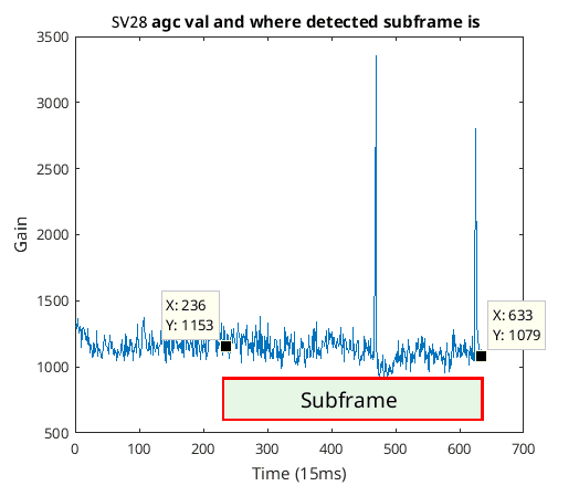 Where packet happened in signal
I was very unlucky and both USB packet drops happened during the subframe. Still, the first half of the subframe looks good and that’s where TLM and HOW are.
The file name that SDRuno created was called DRuno_20201025_223133Z_1575409kHz.wav. We see 20201025_223133Z in that which presumably means 22:31:33 25/10/2020 UTC. I assume this is the time according to my computer when I started recording the signal. The end of the subframe I detected was about 9.495s after the beginning of the recording, therefore, according to my computer the time then should have been about 22:31:42 25/10/2020 UTC or 22:32:00 25/10/2020 GPS after we have added the 18 seconds GPS time is ahead of UTC. This matches to the second which is great. Also the 25th of October 2020 was a Sunday and that also matches. Yay! I can now get the approximate time of the week from the satellites.
I say approximate time because it’s the transmission time of the signal according to the satellite's clock and not the time I receive it. If we consider just the distance to the satellites, the difference is around 66 milliseconds for the 20,000km trip so the time will seem about 66 milliseconds slow by the time I receive it. There are a whole lot of other things to consider too, without considering these things this time is called the uncorrected transmission time sometimes written as or
Going further overview
I was only planning getting the navigation data out of the signals but now I’ve done that the thing on my mind is can I get position solutions from them? To answer that we need to know what’s necessary for calculating one’s position. To do that we need to know where the satellites are and the satellite transmission times to 4 satellites at one instance (aka epoch). The reason for four satellites rather than three is we don’t know the reception time which introduces another variable hence we need another equation which adding a 4th satellite gives us; one satellite per degree of freedom x,y,z and time.
Whilst I am not getting the year or the week of the year from the subframe five that I have received, I know I made the recording on 25/10/2020, so I can use that to resolve the week and year ambiguity so I can get satellite transmission times. That these all have to be at the same epoch we haven’t done yet but the PRN NCO with some ambiguity is the satellite transmission time, so I should be able to do that.
Looking at the satellites of four most powerful signal strengths, only SV7 and SV8 have good signal strengths whilst the other two look like I’m going to have to use SV30 and SV28 which are considerably weaker. Running through all the 6 satellites I detected I managed to detect subframes for 5 of them but not for SV21…
SV7
----Subframe ID=5 TOW: Sun 22:32:00 gps
----100010110000000101000100
----000110100110100000110111
----010001000000011100110101
----001110010000101110011100
----111111010101110000000000
----101000010000110010011000 bad
----011000110101101110110110
----100001011111001000101101
----001000010000111111111011
----111011001111111111101110 bad
----TLM and HOW look ok but if this is a subframe then there are bad words

SV8
----Subframe ID=5 TOW: Sun 22:32:00 gps
----100010110000000101000100
----000110100110100000110111
----010001000000011100110101
----001110010000101110011100
----111111010101110000000000
----101000010000110010011000 bad
----011000110101101110110110
----100001011111001000101101
----001000010000111111111011
----111011001111111111101110 bad
----TLM and HOW look ok but if this is a subframe then there are bad words

SV30
----Subframe ID=5 TOW: Sun 22:32:00 gps
----100010110000000101000100
----000110100110100000110111
----010001000000011100110101
----001110010000101110011100
----111111010101110000000000
----101000010000110010011000 bad
----011000110101101110110110
----100001011111001000101101
----001000010000111111111011
----111011001111111111101101
----TLM and HOW look ok but if this is a subframe then there are bad words

SV28
----Subframe ID=5 TOW: Sun 22:32:00 gps
----100010110000000101000100
----000110100110100000110111
----010001000000011100110101
----001110010000101110011100
----111111010101110000000000
----101000010000110010011000 bad
----011000110101101110110110
----100001011111001000101101
----001000010000111111111011
----111011001111111111101101
----TLM and HOW look ok but if this is a subframe then there are bad words

SV1
----Subframe ID=5 TOW: Sun 22:32:00 gps
----100010110000000101000100
----000110100110100000110111
----010001000000011100110101
----001110010000101110010001 bad
----110010111111101001011101 bad
----101110111110011011001111 bad
----110001101011011101101100 bad
----111101000001101110100101 bad
----010000100001111111110111 bad
----001001100000000000100100 bad
----TLM and HOW look ok but if this is a subframe then there are bad words
Subframe 4 and 5 are exactly the same for all satellites only 1,2, and 3 differ. So even though we don’t get one completely error free subframe I think SVs 7,8,30 and 28 should be okay for the minimum four satellites we need to calculate a position solution. SV1 looks terrible and I don’t think is going to be much use.
To figure out where the satellite was when it transmitted its signals you use ephemerides and the satellite transmission time into a function and it will tell you where the satellite was. These ephemerides are transmitted by the satellites in subframe two and three which we don’t have. Fortunately you can download ephemerides from the Internet as people upload the navigation data to the Internet. The horrendous equations to calculate the satellites position for a given time can be found in “Table 30-II. Broadcast Navigation User Equations (sheet 1 of 4)” of the IS_GPS_200L.pdf document…
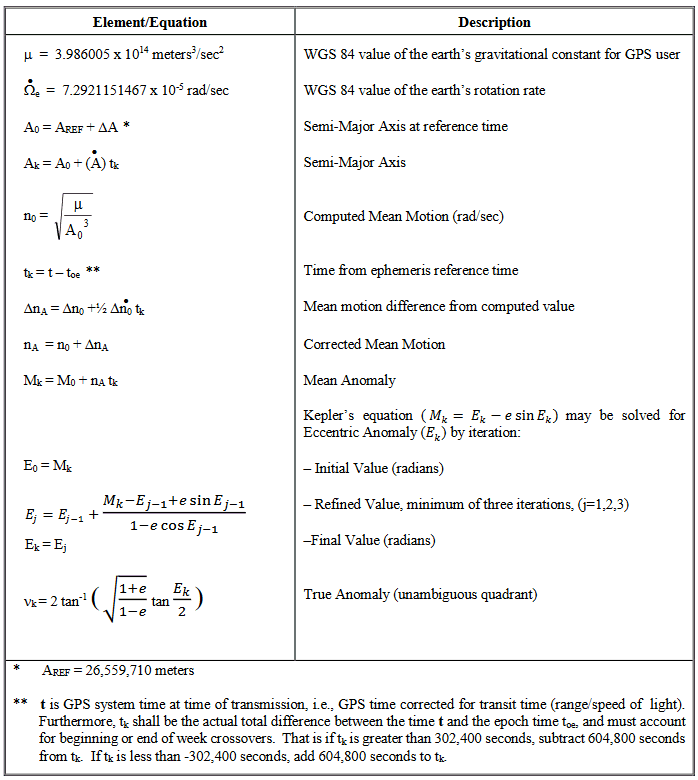 Horrendous equations to calculate the satellites position part 1
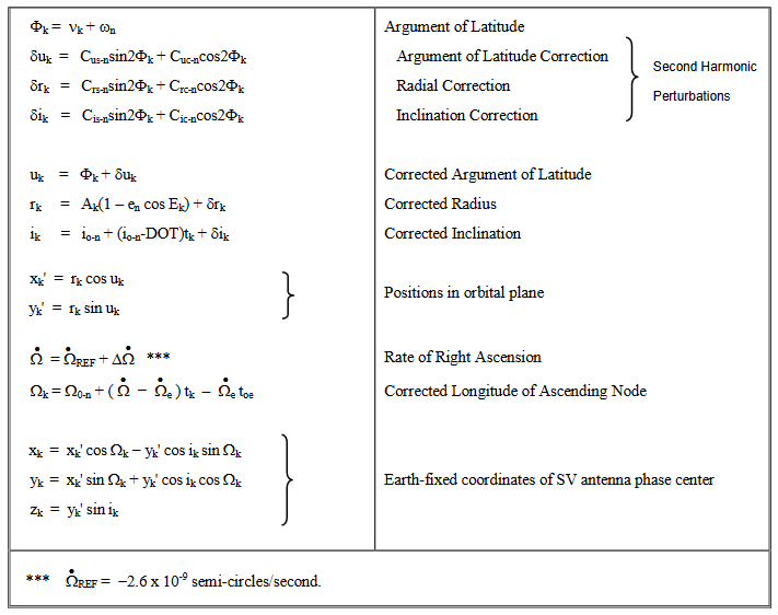 Horrendous equations to calculate the satellites position part 2
Fortunately other people have put these equations into computers so usually you don’t have to bother too much about them.
So it looks like we can use the 12 seconds that Matlab can fit into its memory and with the aid of navigation data that we can download from the Internet calculate a position solution.
PRN tracking again
To calculate the satellite transmission time to all satellites at one epoch we have to look into the PRN NCO a bit more.
When calculating positions using GPS we’ll see people say you need the pseudorange observable and tell you it’s modeled something like…
But less frequently they tell you exactly what the receiver is doing to give you this and that’s what we need to know.
Pseudorange is the same thing as distance if we ignore all the pesky errors such as clock errors etc. That being the case, say humans are living on Mars. A rover on Enceladus, one of Saturn’s moons, sends us a message. This message contains the time and that life is thriving in the liquid water oceans beneath the frozen shell. Forget about the alien life thing, we are more interested in the time part of the message. The message from the rover says it’s 1 PM while our clock says it’s 2 PM…
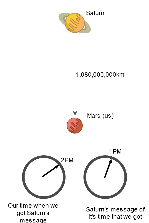 Signal traveling from Enceladus a moon of Saturn to Mars
As it took an hour for the message to get to us and as light travels at 1,080,000,000 km/h that implies the pseudorange is 1,080,000,000 km.
So the pseudorange can be written as follows, where c is the speed of light, the reception time of the message according to the receiver and the transmission time according to the transmitter as received by the receiver (also called uncorrected transmission time) and c is the speed of light…
When talking about the PRN NCO in the tracking block earlier I mentioned that the PRN NCO class does not mod the phase but instead that is left to the owner of the instance to mod it such that the 1st millisecond after a second transition is modded by 1023 chips. The idea is I want the PRN NCO phase to represent the fractional part of the second of the satellites transmission time (i.e. the fractional part of ). Like an analog clock that has hours from 1 to 12 written on it, the PRN NCO when modded as described can be thought of as an analog clock with chips from 0 to 1,022,999 written on it…
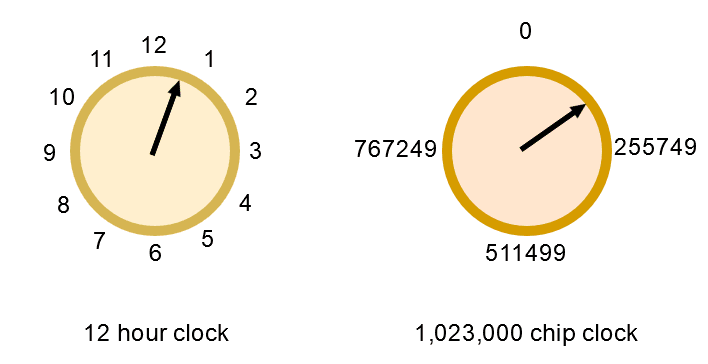 12 hour clock verus a 1,023,000 chip clock
The 12 o’clock goes around once every 12 hours while the 1,023,000 chip clock goes around once every second. Both clocks have an annoying ambiguity. The ambiguity for the 12 hour clock is you don’t know if it’s day or night, what day it is, what month it is, or what year it is. For the 1,023,000 chip clock the ambiguity is it could be any second and you have no idea what the minute, hour, etc. is.
The phase of the PRN NCO looks like an analog clock telling us what the fractional part of is as is in seconds. The integer component of can be obtained from the TOW message and counting full rotations of the phase of the PRN NCO as it passes zero on the clock.
So that solves the mystery of what is, how about ? This one stumped me a bit for a while. is the reception time according to our clock, but where is our clock?, why do we even need a clock when the satellite can provide a better estimate of the current time than we could ever hope to maintain?, and can’t we just say the time is a random number as its something we are wishing to solve for when we calculate our position anyway?
The answer to the first question is we haven’t got one yet. We have to wait until we get the TOW message to get an idea of the time. As that’s our best estimate of the time we would set producing a pseudorange of zero to our first satellite. However we have to use the same for all the other satellites which means if the transmission time received from another satellite was different we would get a different pseudorange for that satellite.
To answer the other questions, we really don’t need a local clock to calculate a position solution and any random number will do for including zero. Why we might want to have a local clock is that the pseudorange would change a lot more slowly with respect to time which is something we can easily plot. It keeps the pseudorange relatively small so we don’t get too much quantization noise. Also with a local clock it could be updated every time we calculated a position solution and thus have a real-time clock that could freewheel between the epochs when we calculate the solution. For our set up where we are using an SDR receiver, a real-time clock that freewheels seems useless to me because we are not connected to the outside world in real time. As for being something easily to plot that doesn’t seem much of a good reason. For quantization noise we can get around that without using the local clock. Anyway, if you know any reason why I should keep a local clock then let me know.
With our ditched local clock the pseudorange measurement becomes…
This is just a scaled version of the transmission time. So the only measurement we have to do at an epoch is take the transmission time for each satellite. However, multiplying the time of week by the speed of light could produce an insanely large number for the poor computer to deal with ( meters) which could produce some nasty quantization noise when we’re trying to keep track of meters. I’d like to get the pseudorange number a lot smaller. To make the pseudorange smaller I’m going to take the fractional component of the reception time before multiplying it by the speed of light…
The curly brackets here are meant to signify that I’m taking the fractional component. Now the fractional component of transmission time is the phase of the PRN NCO converted from chips into seconds or PRN NCO phase divided by 1,023,000 chips; this is a time read from an analog clock.
There is a gotcha here when dealing with this clock/mod stuff. We wish that for any epoch the pseudoranges are consistent. What I mean by this is that a satellite with a more negative pseudorange than another satellite should be closer to us compared to the satellite with the less negative pseudorange…
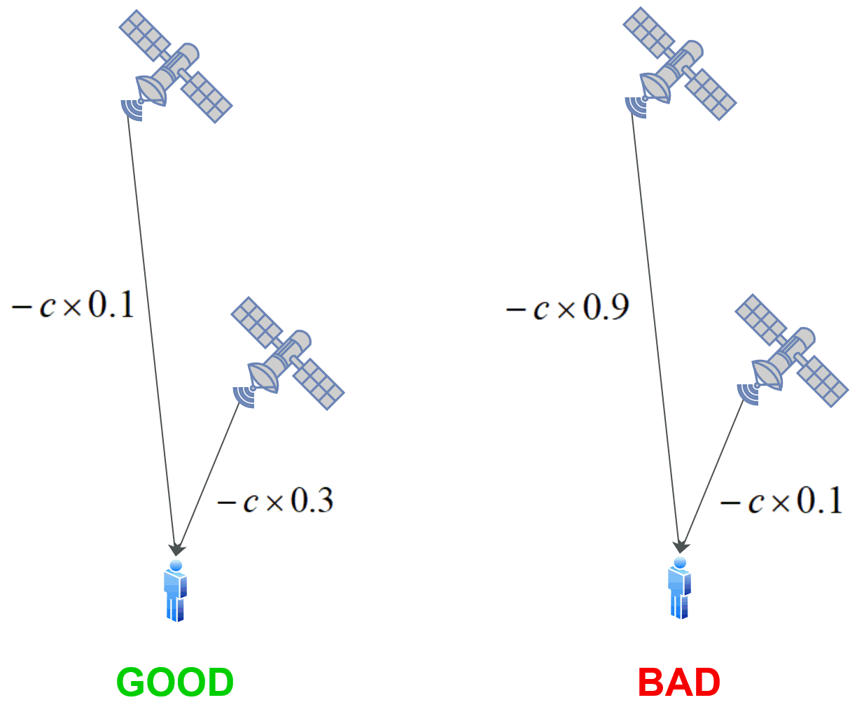 Satellite with more negative pseudorange should be closer
In the figure above mod(0.3-0.1,1)=0.2 but so does mod(0.1-0.9,1)=0.2 and that is a problem when solving the equations to produce a position solution because distance doesn’t make sense in the figure above for the bad epoch. As our clock can only count up to a second the bad epoch is something that is going to be reasonably frequent.
As we can choose to be anything for a given epoch, we can also add any constant we like to each pseudorange measurement for a given epoch. We can use this fact and pick at random one of the satellites in the epoch, forget about the -c for a tick and subtract the fractional component of transmission time from all the satellites in the epoch, add 0.5 to all of them, then mod 1 them, and put the -c back again. That’s more confusing than it sounds but to make clear, doing this to the previous figure we get…
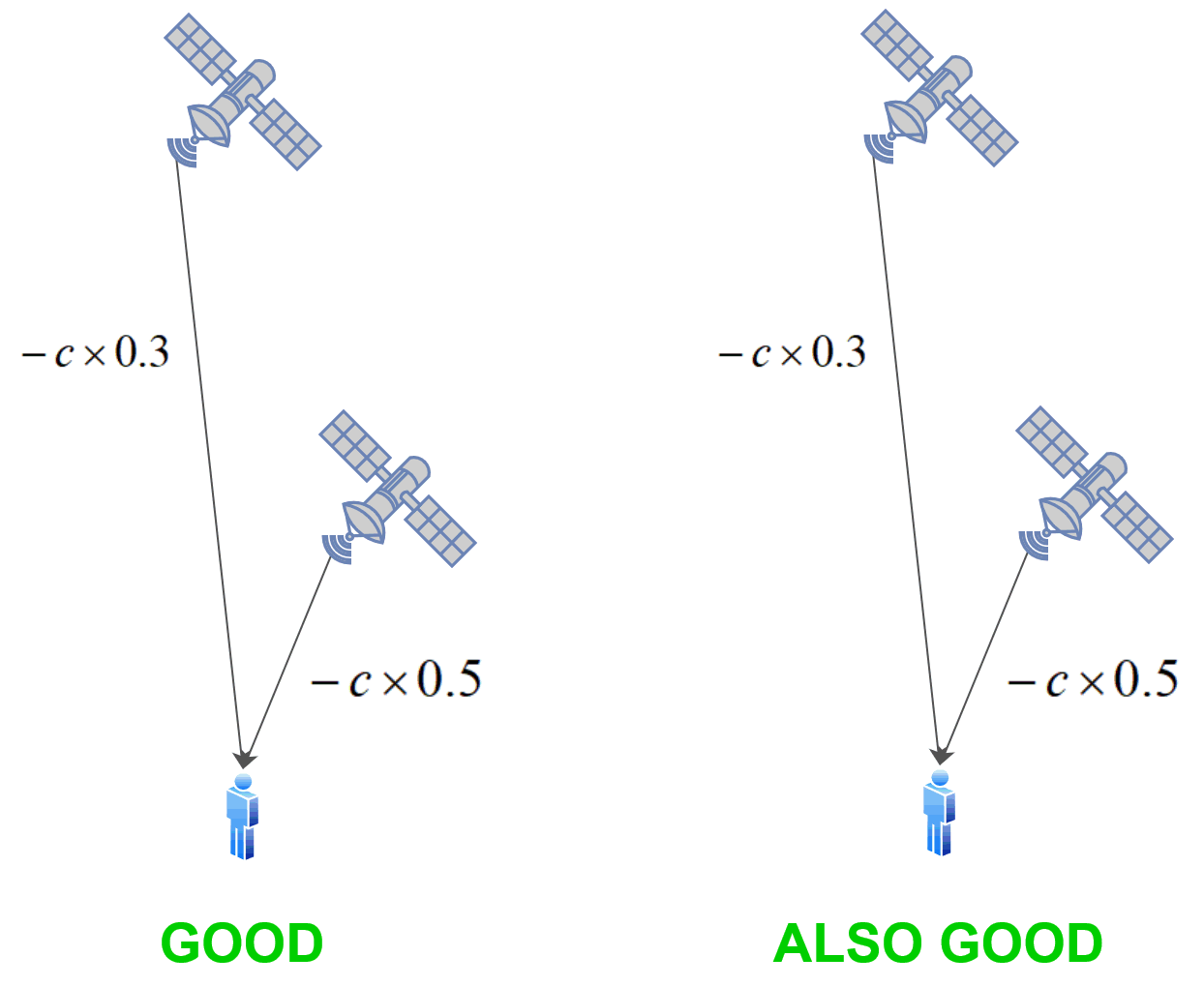 Now fixed the problem. Satellites with more negative pseudoranges are closer
In this instance I have taken the closest satellite in each epoch as the one to subtract. The equations for the first epoch are…
And the second epoch…
Effectively all I’m doing is rotating the clocks such that the hands are more or less about far away as possible from the top of the clock. If you have two 12 hour analog clocks one at 11 and the other at 1, then you could turn them upside down so the hands would point to 5 and 7 respectively…
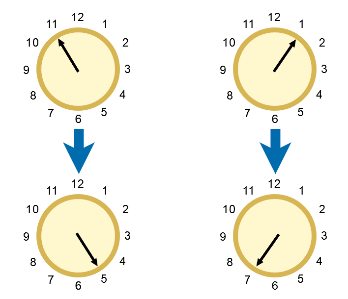 Rotating the clocks so hands are towards the bottom
The details of the rotation don’t really matter as long as the satellites don’t cross the top of the clock. The figure below shows the fractional transmission time of satellites 7,8,30 and 28…
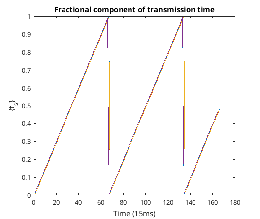 Fractional transmission time
As can be seen from the figure they are all pretty close to one another. If we subtract one of them away from the others they will stop rotating as fast and we will be able to detect any crossing of times at the top of the clock…
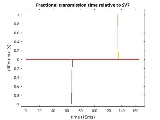 Fractional transmission time relative to SV7
Here we see two crossings which would be bad for calculating solutions. Using the trick of adding 0.5s to all of these lines then mod them by 1s I get the following…
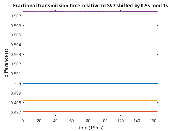 Fractional transmission time relative to SV7 with 0.5s shift and mod 1s
Now we get no crossings at the top of the clock and everything around about half a second. The blue line is SV7 and is exactly at 0.5 and is flat, the others however are not flat. This can be seen in the following figure where I remove the means from all these lines…
fractional_component_of_tx_time_rel_to_sv7_shift_and_mod_mean_removed.png
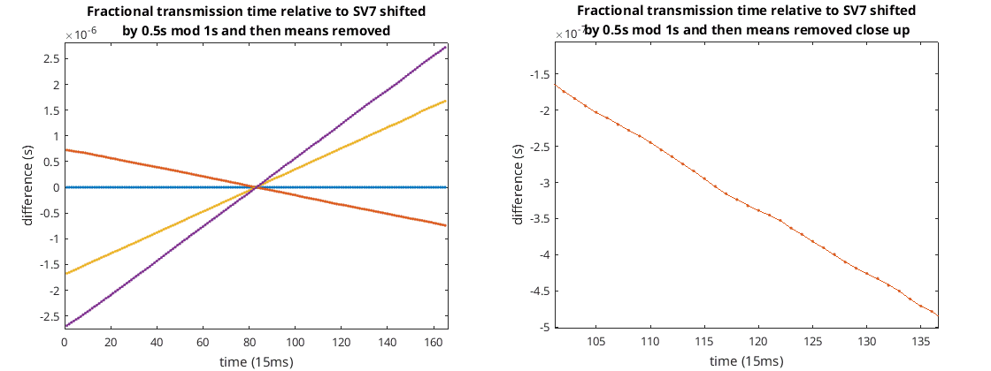 Fractional transmission time relative to SV7 with 0.5s shift, mod 1s, and mean removed
This relative fractional transmission time tells you some satellites are moving towards you relative to SV7 while others are moving away from you relative to SV7 depending on whether or not they have a positive or negative gradient. The figure on the right shows a close-up of one of the lines and as you can see it’s not perfectly smooth.
What maximum relative range between satellites can we get using this trick before we get the possibility of crossings at the top of the clock? If two satellites differ in transmission time received by the user by more than 0.5 seconds we risk crossing the top of the clock as our clock can only cope with one second before it repeats. 0.5 seconds at the speed of light is about 149,896 km that’s big, any two satellites can only be about 40,000 km separated so even though the moon is about 384,400 km away we should still be able to use this trick assuming we can get signals that distance; anyway the geometry at that distance be terrible. Yeah it’ll work anywhere around about the earth.
So our final pseudo-measurement to satellite S is the following…
Where is the fractional transmission time of a random satellite of the epoch.
Right, now, how do we set the phase of the PRN NCO after we have received the subframe? Well, we are processing blockwise so we won’t know about the subframe until the end of the block. The bit_sync class counts the PRN sequence number from 0 to 19 inclusive as described earlier. So, at the end of the block once we have received the subframe we will know the current PRN sequence number and the current PRN NCO phase. If we mod the PRN NCO phase by 1023 chips then add the current PRN sequence number multiplied by 1023 chip we will get the current PRN NCO phase relative to the start of the subframe…
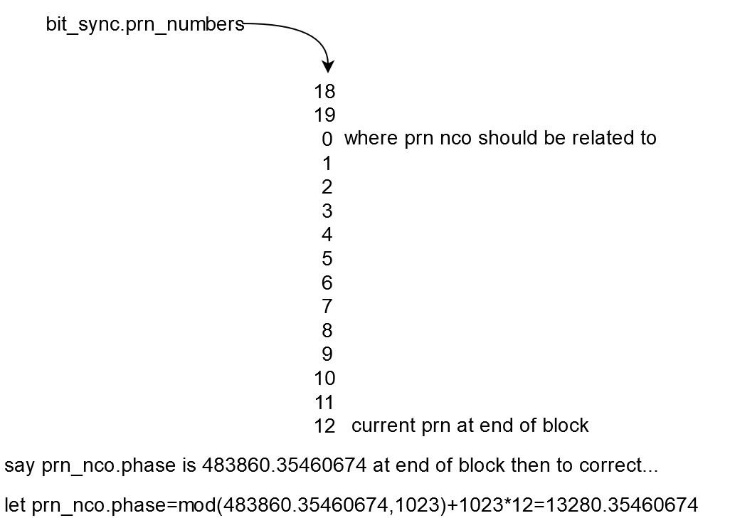 Where PRN NCO zero should be relative to
As we want our PRN NCO phase to have a maximum of one second we have to mod the phase all the time using prn_nco.phase=mod(prn_nco.phase,1023000) as there are 1,023,000 chips per second. If we do both of these things (align with the zeroth prn and mod by 1,023,000 all the time) then…
To keep track of the transmission time itself , we can monitor when prn_nco.phase crosses the top of the clock and add one to each time this happens. Initially we can set to be the time of week obtained from the subframe.
The code for keeping track of both and can be seen below…
%for 1 sec ambi and sync on subframe
if(processed_block_contains_start_of_subframe)
    %phase such that the zero crossing is in the first prn
    prn_nco.phase=mod(prn_nco.phase,prn_nco.prn_len)+1023*bit_sync.prn_numbers(end);%for this to work we cant have more than 20 prns in a block
    %ambi resolved here for sure
    ambi_resolved=true;
else
    if(prn_nco.phase>=(50*20*prn_nco.prn_len))
        sv_tx_int_tow_counter=sv_tx_int_tow_counter+1;%update sec as subframes only happen every 6 secs
    end
    prn_nco.phase=mod(prn_nco.phase,50*20*prn_nco.prn_len);%1sec
end

if(ambi_resolved)
    uncorrected_sv_time_in_seconds=sv_tx_int_tow_counter+((prn_nco.phase/1023)/prns_per_second);
    uncorrected_fractional_sv_time_in_seconds=mod(((prn_nco.phase)/1023)/prns_per_second,1);

    results_for_ls_solving(sv_index).block(end+1)=m;
    results_for_ls_solving(sv_index).ftsv(end+1)=uncorrected_fractional_sv_time_in_seconds;
    results_for_ls_solving(sv_index).tsv(end+1)=uncorrected_sv_time_in_seconds;

    fprintf('block=%d tsv=%.9f\n',m,uncorrected_sv_time_in_seconds);
end
This needs code to signal when the start of the subframe has been detected and the TOW for it…
%bit sync to find start of bits and create a mod 20 counter for the
%prns coming in
bit_sync.bit_sync_update(tracking_output);
%look through each prn for a subframe
processed_block_contains_start_of_subframe=false;
for yy=1:numel(bit_sync.prn_numbers)

    %if prn point has index 0 then we are at the start of a bit
    if(bit_sync.prn_numbers(yy)==0)
        bit_point=bit_sync.bit_points(yy);
        %decode nav bit point
        ca_nav_decoder.update(bit_point);
        %if we have a subframe
        if(ca_nav_decoder.subframe_bad_word_count<10)
            %then we have the time of the start of this prn
            sv_tx_int_tow_counter=ca_nav_decoder.tow;
            processed_block_contains_start_of_subframe=true;
        end

    end

    %unlock if prn corr goes too low
    if(abs(tracking_output (yy))<0.125)
        locked=false;
        ambi_resolved=false;
        fprintf('unlocked at %.3fs\n',block_approx_start_time_wrt_start_of_signal);
    end

end
tracking_output are the 15 points per block of the tracking block output.
You will notice that I have also added code to detect when the signal goes too low by simply deeming loss of lock to be when a normalized PRN correlation is less than 12.5%. I’m sure there are nice ways of doing that but that will do meantime.
So this will keep track of the satellite transmission time with respect to the time of week in seconds, and will also track of the fractional satellite transmission time. In effect this resolves the phase ambiguity of the PRN NCO. Using the two previous code snippets I can attempt to draw them as part of a block diagram…
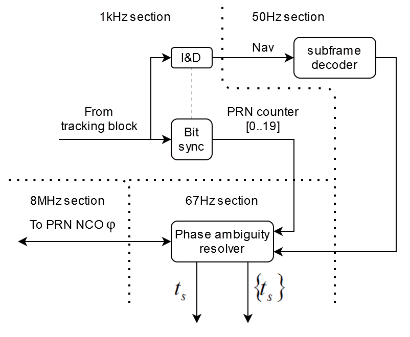 Nav decoder and PRN NCP ambiguity resolver block
The block size I’m using is 15 PRN or an epoch every 15 ms, producing measurements for the satellite transmission time and fractional component of that at 67 Hz. So if I can have four more of these things running at the same time to different satellites and I can download navigation data from the Internet and make use of that I can calculate position solutions.
Putting all the things I've mentioned so far into code for the tracking, from course acquisition to satellite transmission time for any epoch, I can write the code as follows where the input signal is y…
%run through blocks of signal
prn_freq=1000;
for m=1:(12*prn_freq/prns_per_correlation)

    %approx start time in secs
    block_start_sample=samples_per_correlation*m+1;
    block_approx_start_time_wrt_start_of_signal=block_start_sample/Fs;

    %get a block of prn from the prn nco
    prn_nco.next();
    %get a block of signal
    a_org=y(samples_per_correlation*m+1:samples_per_correlation*(m+1));

    %if not locked
    if(~locked)
        %search for signal changing the prn phase given a nominal 1023
        %chips/s chip rate and also the carrier freq
        search_2d.search(a_org);
        %use the search result to adjust the carrier freq,
        %the prn nco phase, and also the agc gain.
        freq_offset=search_2d.frequency_offset_in_hz;
        prn_nco.phase=-(search_2d.chip_offset_in_samples-1)/number_of_samples_per_chip;
        prn_nco.next();
        agc.agc_val=(1/search_2d.correlation);

        %print the search result
        fprintf('--2d search estimation--\n');
        fprintf('frequency_offset_in_hz=%f\n',freq_offset);
        fprintf('prn_nco_phase=%f\n',prn_nco.phase);
        fprintf('agc_val=%f\n',agc.agc_val);

        %say we are locked
        locked=true;

        %say we haven't got the prn ambi resolved
        ambi_resolved=false;
    end

    %carrier_freq_phase,carrier_freq_phase_remainder and
    %carrier_freq_phase_count are for last sample in a_org
    %after the floowoing is done.
    a_slow_spinning=a_org.*exp( ...
        -2*pi*1i*([1:samples_per_correlation].*(freq_offset/Fs)+carrier_freq_phase_remainder) ...
        )';
    carrier_freq_phase=samples_per_correlation*(freq_offset/Fs)+carrier_freq_phase_remainder;
    carrier_freq_phase_remainder=mod(carrier_freq_phase,1);
    carrier_freq_phase_count=carrier_freq_phase_count+round(carrier_freq_phase-carrier_freq_phase_remainder);

    %correlate slow spinning signal with prn block and integrate and dump
    %over each prn not crossing prn boundries
    integrate_and_dump.next(a_slow_spinning.*prn_nco.block,prn_nco.zero_phase_crossing_index);
    %agc for normalized dumped points
    agc.update(integrate_and_dump.dumps./integrate_and_dump.dumps_count);

    %carrier phase tracking
    tracking_output=carrier_tracker.update(agc.signal_out);

    %update carrier frequency (not phase!)
    %unlock if it goes out of bounds
    freq_offset=freq_offset-frequency_offset_gain*carrier_tracker.frequency_offset;
    if(abs(freq_offset)>search_2d.max_freq_offset_to_try_in_hz)
        locked=false;
        ambi_resolved=false;
        fprintf('unlocked at %.3fs due to carrier offset too big\n',block_approx_start_time_wrt_start_of_signal);
    end

    %calc EL chip error
    matched_prn_early=circshift( prn_nco.block, -1 );
    matched_prn_late=circshift( prn_nco.block, +1 );
    chip_tracking_early=(sum(a_slow_spinning.*matched_prn_early)*(agc.agc_val/samples_per_correlation));
    chip_tracking_late=(sum(a_slow_spinning.*matched_prn_late)*(agc.agc_val/samples_per_correlation));
    chip_tracking_error=(abs(chip_tracking_early)-abs(chip_tracking_late));

    %use EL chip error to adjust chip phase. frequency uses either
    %carrier aiding or EL chip error
    prn_nco.phase=prn_nco.phase+chip_tracking_error*chip_tracking_error_phase_gain/2;
    %if carrier aiding
    if(use_carrier_aiding)
        prn_nco.frequency=(tuner_frequency_offset_for_carrier_aiding-freq_offset)/(1540*1000)+1023;
    else
        prn_nco.frequency=prn_nco.frequency+chip_tracking_error*chip_tracking_error_freq_gain;
    end

    %bit sync to find start of bits and create a mod 20 counter for the
    %prns coming in
    bit_sync.bit_sync_update(tracking_output);
    %look through each prn for a subframe
    processed_block_contains_start_of_subframe=false;
    for yy=1:numel(bit_sync.prn_numbers)

        %if prn point has index 0 then we are at the start of a bit
        if(bit_sync.prn_numbers(yy)==0)
            bit_point=bit_sync.bit_points(yy);
            %decode nav bit point
            ca_nav_decoder.update(bit_point);
            %if we have a subframe
            if(ca_nav_decoder.subframe_bad_word_count<10)
                %then we have the time of the start of this prn
                sv_tx_int_tow_counter=ca_nav_decoder.tow;
                processed_block_contains_start_of_subframe=true;
            end

        end

        %unlock if prn corr goes too low
        if(abs(tracking_output(yy))<0.125)
            locked=false;
            ambi_resolved=false;
            fprintf('unlocked at %.3fs\n',block_approx_start_time_wrt_start_of_signal);
        end

    end

    %for 1 sec ambi and sync on subframe
    if(processed_block_contains_start_of_subframe)
        %phase such that the zero crossing is in the first prn
        prn_nco.phase=mod(prn_nco.phase,prn_nco.prn_len)+1023*bit_sync.prn_numbers(end);%for this to work we cant have more than 20 prns in a block
        %ambi resolved here for sure
        ambi_resolved=true;
    else
        if(prn_nco.phase>=(50*20*prn_nco.prn_len))
            sv_tx_int_tow_counter=sv_tx_int_tow_counter+1;%update sec as subframes only happen every 6 secs
        end
        prn_nco.phase=mod(prn_nco.phase,50*20*prn_nco.prn_len);%1sec
    end

    if(ambi_resolved)
        %uncorrected sv time in seconds
        uncorrected_sv_time_in_seconds=sv_tx_int_tow_counter+((prn_nco.phase/1023)/prns_per_second);

        %uncorrected fractional sv time in seconds
        uncorrected_fractional_sv_time_in_seconds=mod(((prn_nco.phase)/1023)/prns_per_second,1);

        results_for_ls_solving(sv_index).block(end+1)=m;
        results_for_ls_solving(sv_index).ftsv(end+1)=uncorrected_fractional_sv_time_in_seconds;
        results_for_ls_solving(sv_index).tsv(end+1)=uncorrected_sv_time_in_seconds;

        fprintf('block=%d tsv=%.9f\n',m,uncorrected_sv_time_in_seconds);

    end

end
So you can see why I made so many classes else this code would be huge and totally unreadable. As it is, it is still quite a big, but manageable. All this code is just for one satellite and I have to repeat it another three times to get enough measurements for a solution. That brings us to calculating satellite positions.
Rinex, SP3, Ephemerides, and satellite positions
To get the position of the satellites accurately enough we need ephemerides. These are broadcast in the navigation data of subframes two and three. As I only have one subframe and that is subframe five, I am going to have to download the ephemerides from the Internet.
The International GNSS Service (IGS) and the National Geodetic Survey (NGS) have broadcast navigation data.
The format of the broadcast navigation data is in RINEX. RINEX (Receiver Independent Exchange Format) is a way of storing various types of GNSS information such as observation and navigation data. For me I’m interested in the broadcast navigation data from GPS for day 299 of 2020. Day 299 of 2020 is the 25th of October 2020 and this conversion can be done from date to day of year with various places on the Internet such as this GPS calendar site . In RIXEX the date is encoded in the file name. I’m looking for a file that has “299” in it and ends with “.20n”, the “n” at the very end of the file name means GPS navigation data. brdc2990.20n is the file I’m looking for, the zero after the 299 signifies that it’s for an entire day. After finding the file and downloading it I had a look at some of it…
     2.11           N: GPS NAV DATA                         RINEX VERSION / TYPE
teqc  2019Feb25     CORS-ADM Account    20201029 15:49:07UTCPGM / RUN BY / DATE
Linux 2.4.21-27.ELsmp|Opteron|gcc|Linux 64|=+               COMMENT
     2.10           N: GPS NAV DATA                         COMMENT
rvacn.e(1404.07)                        2020-10-29T12:33 UTCCOMMENT
This file contains the validated broadcast navigation       COMMENT
messages from the following files:                          COMMENT
abmf2990.20n, abpo2990.20n, albh2990.20n, areq2990.20n,     COMMENT
aspa2990.20n, badg2990.20n, bake2990.20n, barh2990.20n,     COMMENT
bjfs2990.20n, bogt2990.20n, brew2990.20n, brft2990.20n,     COMMENT
chum2990.20n, chur2990.20n, ckis2990.20n, cro12990.20n,     COMMENT
daej2990.20n, dgar2990.20n, drao2990.20n, dubo2990.20n,     COMMENT
fair2990.20n, falk2990.20n, flin2990.20n, glps2990.20n,     COMMENT
glsv2990.20n, gode2990.20n, godz2990.20n, gold2990.20n,     COMMENT
harb2990.20n, hlfx2990.20n, holb2990.20n, hrao2990.20n,     COMMENT
hyde2990.20n, invk2990.20n, irkj2990.20n, jplm2990.20n,     COMMENT
kerg2990.20n, kgni2990.20n, kokb2990.20n, kokv2990.20n,     COMMENT
krgg2990.20n, lmmf2990.20n, lpal2990.20n, mana2990.20n,     COMMENT
maui2990.20n, mcm42990.20n, mdo12990.20n, mdvj2990.20n,     COMMENT
mkea2990.20n, mtka2990.20n, nano2990.20n, nico2990.20n,     COMMENT
nklg2990.20n, nvsk2990.20n, nya12990.20n, nyal2990.20n,     COMMENT
ohi22990.20n, pie12990.20n, pimo2990.20n, pol22990.20n,     COMMENT
polv2990.20n, reun2990.20n, sant2990.20n, sch22990.20n,     COMMENT
scor2990.20n, stjo2990.20n, suth2990.20n, suwn2990.20n,     COMMENT
tehn2990.20n, thti2990.20n, tro12990.20n, unbj2990.20n,     COMMENT
vndp2990.20n, whit2990.20n, will2990.20n, yebe2990.20n,     COMMENT
yell2990.20n, zamb2990.20n                                  COMMENT
    1.2107D-08  0.0000D+00 -1.1921D-07  0.0000D+00          ION ALPHA
    9.4208D+04  0.0000D+00 -1.9661D+05  0.0000D+00          ION BETA
    0.000000000000D+00 6.217248937901D-15   147456     2129 DELTA-UTC: A0,A1,T,W
                                                            END OF HEADER
 1 20 10 24 22  0  0.0 8.133919909596D-04-2.728484105319D-12 0.000000000000D+00
    1.030000000000D+02 1.028125000000D+01 4.109456889660D-09 1.785602150388D+00
    4.023313522339D-07 1.009275927208D-02 4.250556230545D-06 5.153696216583D+03
    5.976000000000D+05-1.825392246246D-07 4.415964148346D-01-2.421438694000D-08
    9.821283218839D-01 3.088437500000D+02 8.291592145637D-01-8.076407843376D-09
    1.771502361613D-10 1.000000000000D+00 2.128000000000D+03 0.000000000000D+00
    2.000000000000D+00 0.000000000000D+00 5.122274000000D-09 1.030000000000D+02
    5.904000000000D+05 4.000000000000D+00
It tells me it’s in RINEX version 2.11 and contains GPS navigation data. The comments say that this file has been produced by merging navigation data received from many stations. After the header you can see the first ephemeris for SV 1 for the time of clock to equal to 22:00h 24/10/2020 GPS. The data in the eight lines for each ephemeris can be seen in the following table…
 +----------------------------------------------------------------------------+
 |                                  TABLE A4                                  |
 |           GPS NAVIGATION MESSAGE FILE - DATA RECORD DESCRIPTION            |
 +--------------------+------------------------------------------+------------+
 |    OBS. RECORD     | DESCRIPTION                              |   FORMAT   |
 +--------------------+------------------------------------------+------------+
 |PRN / EPOCH / SV CLK| - Satellite PRN number                   |     I2,    |
 |                    | - Epoch: Toc - Time of Clock             |            |
 |                    |          year (2 digits, padded with 0   |            |
 |                    |                if necessary)             |  1X,I2.2,  |
 |                    |          month                           |   1X,I2,   |
 |                    |          day                             |   1X,I2,   |
 |                    |          hour                            |   1X,I2,   |
 |                    |          minute                          |   1X,I2,   |
 |                    |          second                          |    F5.1,   |
 |                    | - SV clock bias       (seconds)          |  3D19.12   |
 |                    | - SV clock drift      (sec/sec)          |            |
 |                    | - SV clock drift rate (sec/sec2)         |     *)     |
 +--------------------+------------------------------------------+------------+
 | BROADCAST ORBIT - 1| - IODE Issue of Data, Ephemeris          | 3X,4D19.12 |
 |                    | - Crs                 (meters)           |            |
 |                    | - Delta n             (radians/sec)      |            |
 |                    | - M0                  (radians)          |            |
 +--------------------+------------------------------------------+------------+
 | BROADCAST ORBIT - 2| - Cuc                 (radians)          | 3X,4D19.12 |
 |                    | - e Eccentricity                         |            |
 |                    | - Cus                 (radians)          |            |
 |                    | - sqrt(A)             (sqrt(m))          |            |
 +--------------------+------------------------------------------+------------+
 | BROADCAST ORBIT - 3| - Toe Time of Ephemeris                  | 3X,4D19.12 |
 |                    |                       (sec of GPS week)  |            |
 |                    | - Cic                 (radians)          |            |
 |                    | - OMEGA               (radians)          |            |
 |                    | - CIS                 (radians)          |            |
 +--------------------+------------------------------------------+------------+
 | BROADCAST ORBIT - 4| - i0                  (radians)          | 3X,4D19.12 |
 |                    | - Crc                 (meters)           |            |
 |                    | - omega               (radians)          |            |
 |                    | - OMEGA DOT           (radians/sec)      |            |
 +--------------------+------------------------------------------+------------+
 | BROADCAST ORBIT - 5| - IDOT                (radians/sec)      | 3X,4D19.12 |
 |                    | - Codes on L2 channel                    |            |
 |                    | - GPS Week # (to go with TOE)            |            |
 |                    |   Continuous number, not mod(1024)!      |            |
 |                    | - L2 P data flag                         |            |
 +--------------------+------------------------------------------+------------+
 | BROADCAST ORBIT - 6| - SV accuracy         (meters)           | 3X,4D19.12 |
 |                    | - SV health        (bits 17-22 w 3 sf 1) |            |
 |                    | - TGD                 (seconds)          |            |
 |                    | - IODC Issue of Data, Clock              |            |
 +--------------------+------------------------------------------+------------+
 | BROADCAST ORBIT - 7| - Transmission time of message       **) | 3X,4D19.12 |
 |                    |         (sec of GPS week, derived e.g.   |            |
 |                    |    from Z-count in Hand Over Word (HOW)  |            |
 |                    | - Fit interval        (hours)            |            |
 |                    |         (see ICD-GPS-200, 20.3.4.4)      |            |
 |                    |   Zero if not known                      |            |
 |                    | - spare                                  |            |
 |                    | - spare                                  |            |
 +--------------------+------------------------------------------+------------+
This is from the RINEX 2.11 specification document. While there are newer versions of RINEX, version 2.11 seems to still be the most common but that will probably change with time. As mentioned earlier they are modernizing GPS and they are bringing in a new navigation signal called CNAV (Civil Navigation), and now calling the navigation signal that I am looking at as LNAV (Legacy navigation). As of writing the current status of CNAV is still “Pre-Operational”. As far as I know RINEX 2.11 can’t handle CNAV messages and it will need something like RINEX 4. Anyway version 2.11 is good enough for us. GPS ephemerides are usually updated every two hours valid four 4 hours around what is called the time of ephemeris (TOE).
The Research group of Astronomy and GEomatics (gAGE) has a great way of visualizing RINEX data, they have this page here for visualizing RINEX 2.11 LNAV GPS navigation data where you hover over each element gives you a description of it...
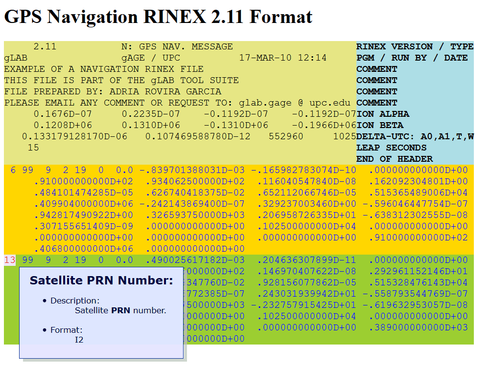 From gAGE's interactive hover over RINEX 2.11 NAV page
To make use of these ephemerides Meysam Mahooti has already written Matlab code to parse RINEX 2.11 NAV files and calculate satellite positions for a given GPS time. However, I had to make a few changes for my needs. I kept his parsef, read_rixex_nav and cal2gpstime functions the same but modified his BroadcastOrbits.m file to fix the week rollover issue that he did not implement which does affect us in New Zealand as it happens around the middle of the day in weekend (over the years it has been a problem surprisingly often). I removed BroadcastOrbits.m and instead created a class that used only the ephemeris with the TOE closest to the requested time. I also added a group delay time correction term for L1 C/A receivers which is documented in the IS-GPS-200 document. The new class I created is as follows…
classdef satposcalulator_class < handle
    %calculate sat positions
    %

    properties
        ECEF;
        sv_clock_bias;
    end

    properties (GetAccess = public , SetAccess = private)

        ephemerides;

        sv_ephemeris;

        svid_;
        m0_;
        dn_;
        e_ ;
        a_ ;
        omg0_;
        i0_ ;
        w_ ;
        odot_;
        idot_;
        cuc_;
        cus_;
        crc_;
        crs_;
        cic_;
        cis_;
        toe_;
        iode_;
        GPS_week_;
        toc_;
        af0_;
        af1_;
        af2_;
        TGD_;

    end

    methods

        function read_nav_file(obj,filename)
            % reads a file or a set of rinex 2.x gps nav files
            if(iscell(filename))
                obj.ephemerides = read_rinex_nav(char(filename(1)));
                for k=2:numel(filename)
                    obj.ephemerides = [obj.ephemerides;read_rinex_nav(char(filename(k)))];
                end
            else
                obj.ephemerides = read_rinex_nav(filename);
            end
        end

        function Reset(obj)
            obj.ECEF=[0,0,0];
            obj.sv_clock_bias=0;
        end

        function obj = satposcalulator_class()
            obj.Reset();
        end

        %towreq is sv time received for L1 receivers if correct_for_sv_time==true else it's gps time
        function [ ECEF ] = getpos(obj,sv,weekreq,towreq,correct_for_sv_time )
            %calculates position of sv given tsv,ephemeris,towreq return ECDF position
            % Input values:
            % sv: sv number
            % weekreq: week of the request in GPS time
            % towreq: time of week request in GPS time
            % correct_for_sv_time: if true then will correct towrequest for relitivity error and sv clock bias
    		% NB all ephemerides need to be in the same week as the request

            %get the closest ephemeride wrt weekreq and towreq.
            %will have week rollover, I think in 2080 due to cal2gpstime
            sv_ephemerides = obj.ephemerides(obj.ephemerides(:,1)==sv,:);
            [~,sv_ephemeride_index]=min(abs((towreq-sv_ephemerides(:,17))+(604800*(weekreq-sv_ephemerides(:,19)))));
            obj.sv_ephemeris=sv_ephemerides(sv_ephemeride_index,:);
            toedelta=(towreq-obj.sv_ephemeris(17));
            assert(abs(toedelta)<(4*60*60),'toe wrt now has to be less than 4 hours');

            %just the best ephemeris for this sv
            ephemeris=obj.sv_ephemeris;

            GM = 3.986005e14;             % earth's universal gravitational [m^3/s^2]
            c = 2.99792458e8;             % speed of light (m/s)
            omegae_dot = 7.2921151467e-5; % earth's rotation rate (rad/sec)

            % initialize constants and variables
            svid = ephemeris(:,1);
            m0   = ephemeris(:,2);
            dn   = ephemeris(:,3);
            e    = ephemeris(:,4);
            a    = (ephemeris(:,5)).^2;
            omg0 = ephemeris(:,6);
            i0   = ephemeris(:,7);
            w    = ephemeris(:,8);
            odot = ephemeris(:,9);
            idot = ephemeris(:,10);
            cuc  = ephemeris(:,11);
            cus  = ephemeris(:,12);
            crc  = ephemeris(:,13);
            crs  = ephemeris(:,14);
            cic  = ephemeris(:,15);
            cis  = ephemeris(:,16);
            toe  = ephemeris(:,17);
            iode = ephemeris(:,18);
            GPS_week = ephemeris(:,19);
            toc=ephemeris(:,20);
            af0= ephemeris(:,21);
            af1= ephemeris(:,22);
            af2= ephemeris(:,23);
            TGD=ephemeris(:,24);

            %done this because matlab doesn't do code highlighting on
            %properites
            obj.svid_=svid;
            obj.m0_=m0;
            obj.dn_=dn;
            obj.e_=e;
            obj.a_=a;
            obj.omg0_=omg0;
            obj.i0_=i0;
            obj.w_=w;
            obj.odot_=odot;
            obj.idot_=idot;
            obj.cuc_=cuc;
            obj.cus_=cus;
            obj.crc_=crc;
            obj.crs_=crs;
            obj.cic_=cic;
            obj.cis_=cis;
            obj.toe_=toe;
            obj.iode_=iode;
            obj.GPS_week_=GPS_week;
            obj.toc_=toc;
            obj.af0_=af0;
            obj.af1_=af1;
            obj.af2_=af2;
            obj.TGD_=TGD;

            nn = size(ephemeris,1);
            for ii = 1:nn

                %deal with week rollover.
                if((towreq-toe(ii))>(604800/2))
                    towreq=towreq-604800;
                elseif((toe(ii)-towreq)>(604800/2))
                    towreq=towreq+604800;
                end

                % Procedure for coordinate calculation
                n0 = sqrt(GM/a(ii)^3); % (rad/s)
                tk = towreq-toe(ii);      % Time from eph ref epoch (s)
                n = n0+dn(ii);         % Corrected mean motion (rad/s)
                M = m0(ii)+n*tk;       % Mean anomaly (rad/s)

                obj.sv_clock_bias=0;
                if(correct_for_sv_time)
                    % Perform Newton-Raphson solution for Eccentric anomaly estimate (rad)
                    NRnext = 0;
                    NR = 1;
                    m = 1;
                    while (abs(NRnext-NR)>1e-15)
                        NR=NRnext;
                        f=NR-e(ii)*sin(NR)-M;
                        f1=1-e(ii)*cos(NR);
                        f2=e(ii)*sin(NR);
                        NRnext=NR-(f/(f1-(f2*f/2*f1)));
                        m=m+1;
                    end
                    E=NRnext; % Eccentric anomaly estimate for computing delta_tr (rad)

                    % Time correction
                    F = -2*sqrt(GM)/c^2; % (s/m^1/2)
                    delta_tr = F*e(ii)*sqrt(a(ii))*sin(E);% relativity eccentricity error
                    delta_tsv = af0(ii)+af1(ii)*(towreq-toe(ii))+delta_tr;%sv clock offset
                    delta_tsv = delta_tsv -TGD;%jonti for L1C/A
                    t = towreq-delta_tsv;
                    obj.sv_clock_bias=delta_tsv;

                    %deal with week rollover.
                    if((t-toe(ii))>(604800/2))
                        t=t-604800;
                    elseif((toe(ii)-t)>(604800/2))
                        t=t+604800;
                    end

                    tk=t-toe(ii);  		 % Time from eph ref epoch (s)
                    M=m0(ii)+n*tk;	     % Mean anomaly (rad/s)
                end

                % Perform Newton-Raphson solution for Eccentric anomaly (rad)
                NRnext=0;
                NR=1;
                m=1;
                while (abs(NRnext-NR)>1e-15)
                    NR=NRnext;
                    f=NR-e(ii)*sin(NR)-M;
                    f1=1-e(ii)*cos(NR);
                    f2=e(ii)*sin(NR);
                    NRnext=NR-(f/(f1-(f2*f/2*f1)));
                    m=m+1;
                end
                E=NRnext; % Eccentric anomaly (rad)
                v = atan2(sqrt(1-e(ii)^2)*sin(E), cos(E)-e(ii));
                phi = v+w(ii);
                u = phi                    + cuc(ii)*cos(2*phi)+cus(ii)*sin(2*phi);
                r = a(ii)*(1-e(ii)*cos(E)) + crc(ii)*cos(2*phi)+crs(ii)*sin(2*phi);
                i = i0(ii)+idot(ii)*tk     + cic(ii)*cos(2*phi)+cis(ii)*sin(2*phi);
                Omega = omg0(ii)+(odot(ii)-omegae_dot)*tk-omegae_dot*toe(ii);
                x1 = cos(u)*r;
                y1 = sin(u)*r;

                % ECEF coordinates
                assert(svid(ii)==sv,"error sv doesn't match");
                ECEF(1,ii) = x1*cos(Omega)-y1*cos(i)*sin(Omega);
                ECEF(2,ii) = x1*sin(Omega)+y1*cos(i)*cos(Omega);
                ECEF(3,ii) = y1*sin(i);

            end

            obj.ECEF=ECEF;

        end

    end

end
Once it’s initialized calculating the satellite positions done by calling the getpos(obj,sv,weekreq,towreq,correct_for_sv_time ) function.
For me looking through the RINEX NAV file for the satellite SV 7 I see the following ephemeris has a TOE of 79184 seconds GPS while the recording satellites I made was around 81120 seconds GPS; that’s about 30 minutes difference so it is the ephemeris that I need to use for SV 7…
7 20 10 25 21 59 44.0-4.009623080492D-04-7.844391802792D-12 0.000000000000D+00
    4.800000000000D+01 4.618750000000D+01 5.119141804232D-09 1.141822219307D+00
    2.570450305939D-06 1.422125415411D-02 6.934627890587D-06 5.153633096695D+03
    7.918400000000D+04-1.117587089539D-07-2.819485670004D+00 2.086162567139D-07
    9.528126446312D-01 2.453437500000D+02-2.361589094236D+00-8.528569534868D-09
    7.000291590243D-11 1.000000000000D+00 2.129000000000D+03 0.000000000000D+00
    2.000000000000D+00 0.000000000000D+00-1.117587089539D-08 4.800000000000D+01
    7.201800000000D+04 4.000000000000D+00
For a test I’m going to calculate the satellite position of SV7 at 22:30 GPS (81000 seconds GPS). As this is is a test and is GPS time I don’t need to make any corrections so I will set correct_for_sv_time to false in the getpos function. Putting in SV7 week 2129 and time of week request to 81000 I get the following satellite position for SV7…
satposcalc.getpos(7,2129,81000,false)

ans =

         -20083290.1736816
            -832972.168008
         -17274143.7570931
The output of this is in ECEF coordinate system which is an orthogonal one where the z axis goes through the North Pole, the x axis comes out the equator at zero longitude, and finally the last one y also comes out the equator but with a longitude of 90° east. ECEF is in meters and (0,0,0) is in the center of the earth.
The reason I chose 22:30 GPS to calculate the location is that I can use SP3 files to check the accuracy of this result. SP3 files are files that contain the location of satellites for specific times. I downloaded igr21290.sp3 from the same folder I downloaded the brdc2990.20n file from and is for the same day. The following shows the entry for SV7 at 22:30 IGS (almost the same thing as GPS time)…
*  2020 10 25 22 30  0.00000000
PG07 -20083.290238   -832.972552 -17274.143854   -400.983366  8  7  6 113
The format of this entry can be seen in SP3 Version C specification.
So this means the SP3 file predicts that the satellite should be at (-20083290.238,-832972.552,-17274143.854) meters with a clock offset of -400.983366 microseconds, an x,y,z standard deviation of (8,7,6) mm and a clock standard deviation of 16.29ps.
Comparing the SP3 result with the one obtained from the RINEX file we get a difference of (0.064,0.384,0.097) meters and an absolute difference of 0.40 meters. So that’s reasonable I guess and looks like the code that calculates satellite positions from RINEX LNAV data is working as it should.
Corrections corrections corrections
One fascinating thing about GNSS is it allows a way to see phenomena one does not see on a day-to-day basis. If one does not take into account these strange phenomena one does not get a very good GPS position solution.
You get people who say “GPS wouldn’t work without general relativity”. That’s a bit of an odd thing to say and I don’t think quite make sense. I think a more accurate thing to say would be GPS wouldn’t work well without lots of corrections.
I was watching an episode of numberfile where the guy was going through mistakes people make when talking about general relativity and GPS came up. I’m not sure I totally understood what he was on about but he mentioned that clocks on GPS satellites run a bit fast as seen from Earth and that is taken into account by the satellites by running them a bit slow so that from Earth they seem to be running at about the correct speed. Indeed, page 14 of the IS-GPS-200L document says that the satellite signals are derived from a clock that is nominally 10.23 MHz from earth but runs at about 10.2299999954326 MHz on the satellite itself. That’s correction number one, we didn’t even have to do it ourselves and is taken care of by the kind folks that build these satellites. The numberfile guy then mentioned that the earth not being a perfect sphere causes everyone at sea level to measure the same time which was interesting and something I didn’t know. So do we personally have to account for any relativistic effects? Well yes, there is, the IS-GPS-200L document page 95 says there is a relativistic effect you should correct for; that’s the second correction and we have to do it ourselves. According to page 41 of http://www2.unb.ca/gge/Resources/gpsworld.nov-dec91.corr.pdf it’s due to the eccentricity of the satellite’s orbit.
The satellites have a few clocks on them that are pretty accurate. I found it a bit hard to find information on what the clocks are on board where https://gssc.esa.int/navipedia/index.php/GPS_Space_Segment says for Block IIF satellites use two rubidium and one cesium are used, while http://www2.unb.ca/gge/Resources/gpsworld.nov-dec91.corr.pdf says “GPS Block II satellite contains two cesium clocks”. Cesium clocks are an order of magnitude more accurate than rubidium so I would’ve thought having only one cesium clock would be a bit risky. Anyway while these clocks are accurate they aren’t perfect and they do have an offset, a drift, and a drift of a drift; these values are calculated presumably by people on earth and transmitted by the satellites in the ephemerides as and respectively. Plotting only this correction for SV7 for 24 hours on the first day of week 2129 we get the following plot…
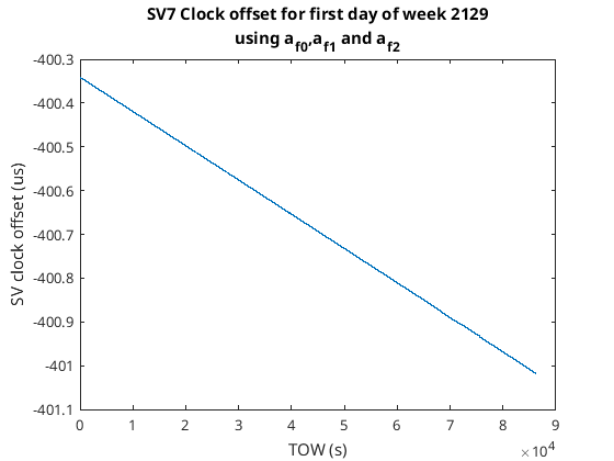 Clock correction as transmitted by the satellite
It’s just a straight line, this is because all ephemerides I’ve ever seen have , I’m not sure if they ever use the term. Anyway, this is a huge correction and the largest we are going to see, at the speed of light this is a range correction of around 120 km. Now, how about we add the relativistic correction to that due to the eccentricity of the orbit…
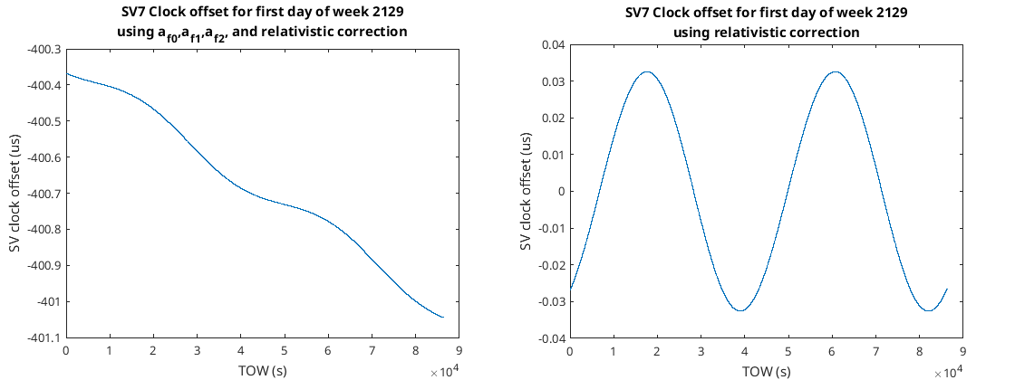 Clock correction as transmitted by the satellite and relativistic correction
The above figure on the left is both corrections added together while the above figure on the right is just the relativistic correction alone. The relativistic correction on its own accounts for a range correction of 9 m; whilst not super huge it still is a significant amount. You can see the figure on the right almost exactly repeats itself every 12 hours that’s because that’s the GPS orbital period. How does this relativistic correction depend on satellite distance? As everything repeats after 12 hours let’s just look at 12 hours for SV7 and SV8…
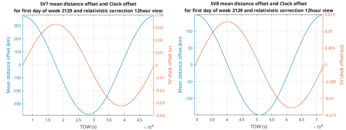 Satellite mean distance offset and relativistic correction
So that’s weird and not quite what I expected. It seems when the satellite is at apogee or perigee (as far as it can be away and as close as it can be to us respectively) the relativistic correction is zero, when going from apogee to perigee the clock offset is positive, and when going from perigee to apogee the clock offset is negative. So the radial velocity of the satellite with respect to the center of the earth that seems to change the relativistic correction a lot; let’s plot that…
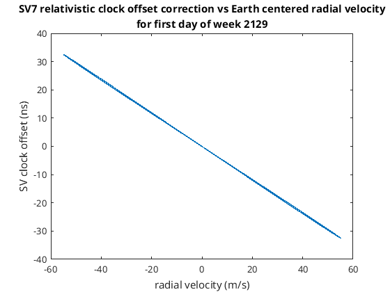 Relativistic correction versus radial velocity
Yup it does but as you can see that’s not the only thing that changes it. Looking at the IS-GPS-200L document this relativistic correction can be written as...
Where is the clock offset caused due to this relativistic phenomena, the location of the satellite relative to the center of the earth, the velocity of the satellite, and the speed of light. Another way to describe this is…
Where is the distance to the satellite from the center of the earth and is the radial velocity of the satellite. This is why it seems to be approximately proportional to the radial velocity as is big and is small. Plotting versus I get the following…
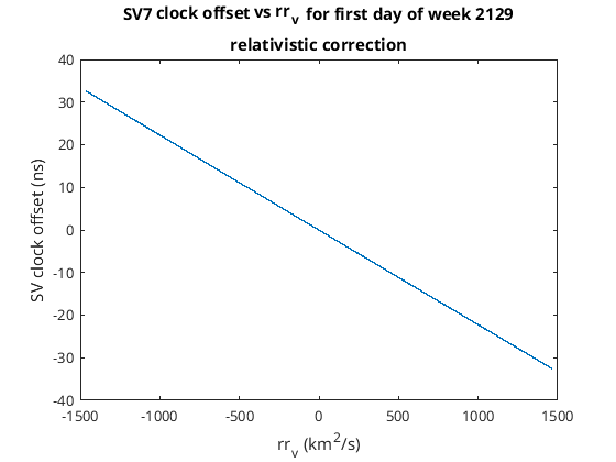 Relativistic correction versus distance times radial velocity
This time I get an almost perfect match and the plot seems as if it’s a straight line.
This open access as Journal at https://link.springer.com/content/pdf/10.12942%2Flrr-2003-1.pdf mentions this correction and goes into great depth about other GPS corrections too; it’s well worth a read. The current correction I’m looking at they call “The eccentricity correction”.
The third correction I’m going to make is one using the ephemeris entry called TGD (total group delay). Page 96 of the IS_GPS_200L document mentions that single frequency users such as myself need to modify the received satellite transmission time using this value. For the L1 C/A signal that I’m using it says that I need to subtract this from the clock offset. It seems that this correction has something to do with individual satellite itself and something calculated when the satellite is manufactured although it may get occasionally updated during operation. I’m not sure what this correction is all about but I’ll apply it as directed.
That should finish off the time corrections. From the satellite calculation section the listing of the Matlab code for the class you may have noticed the following…
if(correct_for_sv_time)
    % Perform Newton-Raphson solution for Eccentric anomaly estimate (rad)
    NRnext = 0;
    NR = 1;
    m = 1;
    while (abs(NRnext-NR)>1e-15)
        NR=NRnext;
        f=NR-e(ii)*sin(NR)-M;
        f1=1-e(ii)*cos(NR);
        f2=e(ii)*sin(NR);
        NRnext=NR-(f/(f1-(f2*f/2*f1)));
        m=m+1;
    end
    E=NRnext; % Eccentric anomaly estimate for computing delta_tr (rad)

    % Time correction
    F = -2*sqrt(GM)/c^2; % (s/m^1/2)
    delta_tr = F*e(ii)*sqrt(a(ii))*sin(E);% relativity eccentricity error
    delta_tsv = af0(ii)+af1(ii)*(towreq-toe(ii))+af2(ii)*(towreq-toe(ii))^2+delta_tr;%sv clock offset
    delta_tsv = delta_tsv -TGD;%jonti for L1C/A
    t = towreq-delta_tsv;
    obj.sv_clock_bias=delta_tsv;

    %deal with week rollover.
    if((t-toe(ii))>(604800/2))
        t=t-604800;
    elseif((toe(ii)-t)>(604800/2))
        t=t+604800;
    end

    tk=t-toe(ii);  		 % Time from eph ref epoch (s)
    M=m0(ii)+n*tk;	     % Mean anomaly (rad/s)
end
This is the part of the code that performs the time corrections I’ve discussed so far…
% Time correction
F = -2*sqrt(GM)/c^2; % (s/m^1/2)
delta_tr = F*e(ii)*sqrt(a(ii))*sin(E);% relativity eccentricity error
delta_tsv = af0(ii)+af1(ii)*(towreq-toe(ii))+af2(ii)*(towreq-toe(ii))^2+delta_tr;%sv clock offset
delta_tsv = delta_tsv -TGD;%jonti for L1C/A
t = towreq-delta_tsv;
obj.sv_clock_bias=delta_tsv;
It takes into account the relativity eccentricity error, the clock offset as transmitted by the satellite, and also the total group delay transmitted by the satellite; is not calculated the satellite clock error (aka delta_tsv) reasonably accurately. Next what happens to our pseudo-range?
Our pseudorange model is still…
And we have the following number filed away in a vector somewhere…
So we can add our estimate of to the pseudorange and create a new pseudorange which is different from the previous one…
For now I’m going to ignore the tropospheric, ionospheric, multipath errors, miscellaneous errors as I’m finding this quite tiring…
Are we done making corrections? No, there’s one more that if I don’t do it I’ll end up about 30 m to the east. I am not too sure of the name I think it’s called the Sagnac effect but to me it looks like the Coriolis effect. Whatever it is, it comes about due to using the ECEF rotating reference frame. Imagine the following. We are on the equator and there is a satellite directly overhead in a geostationary orbit. The satellite throws us a ball which takes six hours to get to us, what sort of path does it take? Well, the satellite has to throw the ball to us such that when it hits the earth we will be in that location, that’s not where we are now, that’s where we will be in six hours time. In six hours we will have rotated about one quarter of a revolution around the center of the earth; therefore the satellite has to throw the ball to the side of the Earth. This is made a lot clearer by just showing you the following gif, where the left animation shows the ball’s trajectory in the ECEF frame while the right animation shows the ball’s trajectory in an ECI frame…
 Throwing a ball from a geostationary satellite that takes 6 hours to reach a person on Earth in two different reference frames
These two animations are exactly the same I just rotated the one on the right to make it look like it wasn’t rotating to create the one on the left.
I believe the same kind of thing happens to the satellite signals as they make their merry way to us on Earth. It’s very weird that in our ECEF frame that we live in, signals from satellites don’t seem to go in straight lines; weird.
Looking at page 106 and 107 of the IS-GPS-200L document talk about geometric range and an ECI coordinate system. What I make from this is that if the epoch time in GPS is (the time now when we want to calculate a position solution) then you can rotate the satellite which is at GPS time, both will be in ECI frame so you can calculate the range, calculated a position solution, and as you didn’t rotate yourself (the ECI frame is coincident with the ECEF frame at time ) you don’t have to bother about converting back into ECEF frame. Basically just rotate satellites clockwise a bit before you start finding a position solution. Anyway I’ll get onto that later when describing how to calculate the position solution.
As you can see the number of corrections to make can be enormous. I have just done the basic corrections that will get a reasonable pseudorange and transmission time.
Position solutions
The distance to a satellite from a user located at can be written as follows.
Or
Where
And
The pseudorange measurement (we have this thing the corrections) is related to this distance via the user’s clock error as written below where is the speed of light and is the user’s clock error.
This is a nonlinear equation with respect to and is a hassle to solve.
If we forget about the notation for a minute and instead imagine ourselves on a hill. The ground directly beneath our feet might be sloping but to a pretty good approximation it’s not undulating or doing anything weird. The undulating weird things are only apparent over distances a long way away from our feet. So we have a way of modeling points on the ground close to our feet quite accurately if we just treat the ground around our feet as a plane. The nice thing about this is that planes (or other dimension equivalents) are linear and easy to deal with. This linearization of some interesting function say of height above sea level can be written as follows where is where we are currently standing.
This is a truncated Taylor expansion. is the slope of the ground beneath our feet while is the location we wish to investigate.
Back to satellites we can use the same linearization of the pseudo-range equation…
We simplify a little…
Everything with a hat on it is a guess. It might look more complicated but it’s a linear function with respect to its input variables. With a bit of tidying up it can be made to look very simple…
Where
Then if we get some more of these pseudo-ranges from other satellites the same time we can write this as the following…
Where
Then use least-squares to solve for , iterate and we are done.
As mentioned in the last section the satellite is first rotated using the distance to the guessed solution so we have an ECI frame that is coincident with the ECEF frame at the time we wish to have a solution. Also as mentioned in the last section transmission time has to be corrected for and so does the pseudo range. In code finding solutions look like the following for me…
%find min and max epochs
min_block=inf;
max_block=-inf;
for sv_index=1:numel(svs)
    minb=min(results_for_ls_solving(sv_index).block);
    maxb=max(results_for_ls_solving(sv_index).block);
    if(minb<min_block)min_block=minb;end
    if(maxb>max_block)max_block=maxb;end
end

%run through each epoch one at a time solving for position
sols=zeros(4,0);
solution_epoch=[];
for epoch=min_block:max_block
    %find all svs that have this epoch
    lssv=[];
    lsrho=[];
    lstsv=[];
    for sv_index=1:numel(svs)
        idx=find(results_for_ls_solving(sv_index).block==epoch);
        if(isempty(idx))continue;end

        lssv(end+1)=results_for_ls_solving(sv_index).sv;
        lsrho(end+1)=results_for_ls_solving(sv_index).ftsv(idx);
        lstsv(end+1)=results_for_ls_solving(sv_index).tsv(idx);
    end
    %we need at least 4 svs per epoch to solve
    if(numel(lssv)<4)continue;end

    %create rho from ftsv by moving hands to bottom of clock, mod by 1 then multiply by -c
    shift_val=lsrho(1);
    for sv_index=1:numel(lssv)
        lsrho(sv_index)=-c*mod(lsrho(sv_index)-shift_val+0.5,1);%no local prn
    end

    %fill in sv locations and make rho corrections
    lsS=zeros(numel(lssv),3);
    for sv_index=1:numel(lssv)
        sv=lssv(sv_index);
        rho=lsrho(sv_index);
        tsv=lstsv(sv_index);
        satposcalc.getpos(sv,weekreq,tsv,true);
        lsS(sv_index,:)=satposcalc.ECEF;
        lsrho(sv_index)=rho+c*satposcalc.sv_clock_bias;%pseudorange correction
    end

    lsS_org=lsS;
    rho_measured=lsrho';
    guessed_sol=[0;0;0;0];

    A=zeros(numel(lssv),4);
    rho_expected=zeros(numel(lssv),1);
    for k=1:10

        %rotate svs back for earth rotation while svs are transmitting
        omegae_dot = 7.2921151467e-5; % earth's rotation rate (rad/sec)
        for sv_index=1:numel(lssv)
            propagation_distance_in_meters=norm((lsS_org(sv_index,:)'-guessed_sol(1:3))');
            gamma=omegae_dot*propagation_distance_in_meters/c;
            rotate3d=[...
                cos(gamma),sin(gamma),0;...
                -sin(gamma),cos(gamma),0;...
                0,0,1;...
                ];
            lsS(sv_index,:)=(rotate3d*lsS_org(sv_index,:)')';
        end

        %create A
        for sv_index=1:numel(lssv)
            A(sv_index,:)=[(lsS(sv_index,:)'-guessed_sol(1:3))'/norm(lsS(sv_index,:)'-guessed_sol(1:3)),-1];
        end

        %create rho
        for sv_index=1:numel(lssv)
            rho_expected(sv_index)=(norm(guessed_sol(1:3)-lsS(sv_index,:)')+guessed_sol(4));
        end

        %calc expected rho
        delta_rho=rho_expected-rho_measured;

        %this is least squares
        %solve for delta_x --> A*delta_x=delta_rho
        delta_x=A\delta_rho;

        %update guessed_sol as we just solved for delta_X
        guessed_sol=guessed_sol+delta_x;

    end

    sols(:,end+1)=guessed_sol;
    solution_epoch(end+1)=epoch;
So it’s a bit weird, you effectively guess a solution and progressively make better guesses. You might find http://indico.ictp.it/event/a12180/session/21/contribution/12/material/0/0.pdf a useful resource which are some slides about corrections and obtaining positions solutions.
Finally I convert the ECEF coordinates into North East Up coordinates (NEU) using the following…
%calc neu sols rel to actual_sol
sols_neu=sols;
ref_loc=ecef2lla(actual_sol(1:3)');%reference location
for k=1:size(sols,2)
[north,east,up]=ecef2ned(sols(1,k),sols(2,k),sols(3,k),ref_loc(1),ref_loc(2),ref_loc(3),wgs84Ellipsoid);
up=-up;
sols_neu(:,k)=[north;east;up;sols(4,k)];
end
In this case actual_sol is the reference location for the NEU solutions and I obtained from Google Earth. With that I can then plot the solutions which gives me a bird’s eye view, I can also plot the absolute distance between position solution and the location obtained from Google Earth; both of these can be seen in the following two figures…
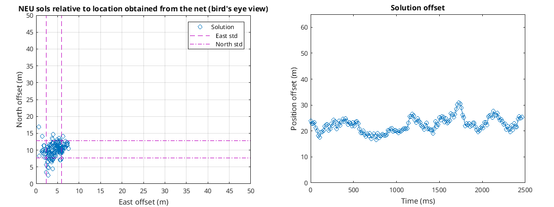 Position solutions in NEU format with reference obtained from Google Earth
So here in getting solutions at a rate of 67Hz, and East standard deviation of 1.8m, and North standard deviation of 2.5m, a total median offset of 22.2m, and a North East median offset of (4.3,10.2) meters. So I’m pretty pleased with that, and the answer is yes, if you record 19 seconds of seemingly blank 1575.42 MHz frequencies using an SDR receiver you can obtain both time and position solution with the help of the Internet.
Position solution accuracy without corrections
So now I have the best solution I can currently get, how about I remove one correction at a time and see the effect this has on the position solutions?
Removing the Sagnac correction…
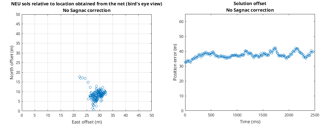 Position solutions without Sagnac correction
Without the Sagnac correction moves me 30 m to the East.
Removing the TGD correction instead…
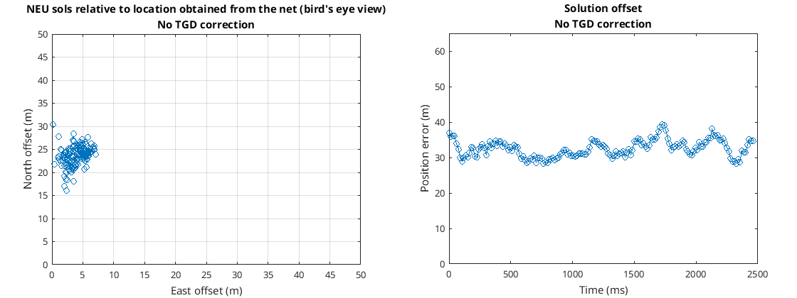 Position solutions without TGD correction
That seems to move me 15 m to the North.
Removing the relativistic eccentricity correction instead…
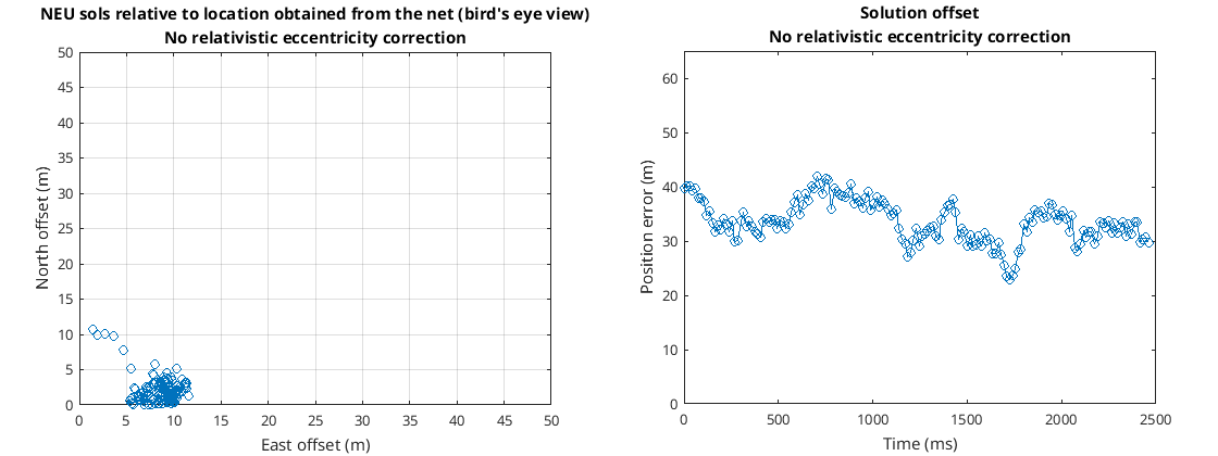 Position solutions without relativistic eccentricity correction
That seems to move me 5 m to the North and 10m to the South.
Removing the clock offset as transmitted by the ephemerides instead…
 Position solutions without ephemeris clock correction
Hmmm, that moves me about 100 km north and 700 km beneath the planet. Still, it shows that I’m in New Zealand.
Here’s a table of the correction removed, the total standard deviation and the median distance to the location is obtained from Google Earth…
| Correction removed | Solution standard deviation | Median solution distance from one obtained from Google Earth |
|---|---|---|
| None | 2.7m | 22.2m |
| Sagnac | 1.9m | 37.2m |
| TGD | 2.4m | 32.5m |
| Relativistic eccentricity | 3.8m | 33.5m |
| Clock ephemerides | 10.1m | 713km |
So from this table we see that using all the corrections produces a solution with the least distance to the reference Google Earth position but it doesn’t have the least standard deviation; that prize goes to not applying the Sagnac correction. I would’ve thought that using all the corrections I would’ve got the lowest standard deviation; anyway this is what I got.
Ionospheric correction
Okay let’s try an ionospheric correction using the Klobuchar model. The pseudorange model is…
The stands for ionospheric error. With a single frequency receiver it's not an easy thing to remove but I’ll give it a go. I changed the read RINEX function to retrieve the alpha and beta values that are sent in the navigation data…
alpha=zeros(1,4);
beta=zeros(1,4);

% look through header looking for alpha and beta
end_of_header = 0;
while end_of_header == 0
    current_line = fgetl(fid);
    % if ION ALPHA
    if strfind(current_line,'ION ALPHA')
        [alpha(1),alpha(2),alpha(3),alpha(4)] = parsef(current_line, {'D14.4','D12.4','D12.4','D12.4'});
    end
    % if ION BETA
    if strfind(current_line,'ION BETA')
        [beta(1),beta(2),beta(3),beta(4)] = parsef(current_line, {'D14.4','D12.4','D12.4','D12.4'});
    end
    if strfind(current_line,'END OF HEADER')
        end_of_header=1;
    end
end
In the satellite position calculator returns them…
obj.alpha_=ephemeris(:,25:28);
obj.beta_=ephemeris(:,29:32);
Then when correcting the pseudorange I subtract ionospheric error in meters from the pseudorange…
%ion estimate
if(sum(isnan(approx_receiver_pos))==0)
    [azimuth,elev,slantRange] = ecef2aer(satposcalc.ECEF(1),satposcalc.ECEF(2),satposcalc.ECEF(3),lla_ref(1),lla_ref(2),lla_ref(3),wgs84Ellipsoid('meters'));
    Ion_estimate=klobuchar(lla_ref(1),lla_ref(2),elev,azimuth,tsv,satposcalc.alpha_,satposcalc.beta_);
end

lsrho(sv_index)=rho+c*satposcalc.sv_clock_bias-Ion_estimate;
Here I use the function klobuchar that Meysam Mahooti also wrote that can be found here https://au.mathworks.com/matlabcentral/fileexchange/59530-klobuchar-ionospheric-delay-model . This time using this new correction I obtain the following…
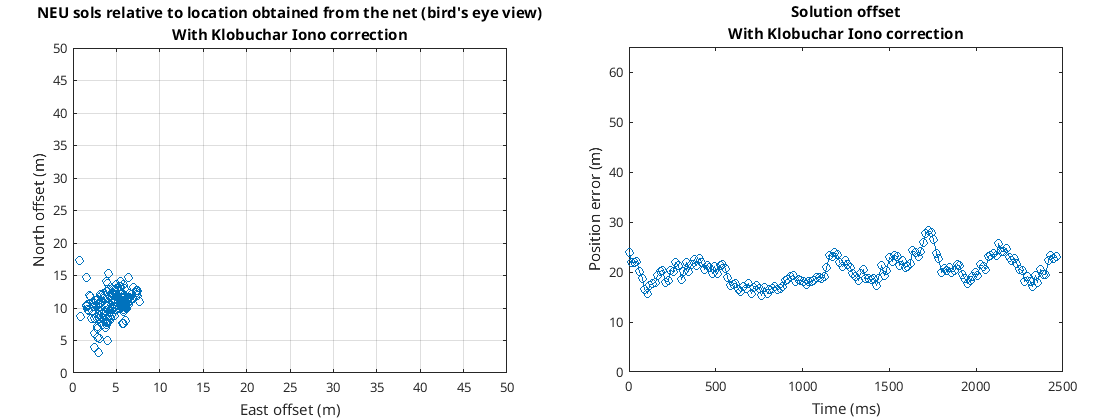 Position solutions with Klobuchar ionosphere correction and all pervious corrections applied
It doesn’t significantly change but the new solution standard deviation is 2.6m and the median solution distance from the one obtained from Google Earth is 20.2m. That’s 0.1 m better standard deviation and 2 meters closer to the one obtained from Google Earth.
Two more recordings
During this write up, Darren’s RSP1A arrived, thanks very much for that. This SDR receiver features better out of band signal rejection, a more stable oscillator, and best of all it has a t-bias so no more having to cobble together external hardware to power the active antenna.
I took this receiver outside and over two consecutive days made two recordings; one for each day. Each of these recordings was about 30 seconds long. The following figure using Google Earth shows approximately where the antenna was for the first and second day marked with one and two respectively.
 Image of where the two recordings were made over the two separate days
The resolution is terrible but without using a drone to take a picture of about my house that’s as good an image as I can get. The picture is orientated with north at the top and east towards the right.
I figured out SDRuno a little and found that the 11 kHz offset I measured earlier on is actually one of the settings in SDRuno. I also noticed that there is a setting for choosing between isochronous and bulk transfer for the USB interface. I changed that to bulk transfer as that should be less likely for USB packet drops to happen as I think it has guaranteed transfers rather than isochronous which is a fire and forget transfer method I believe. With this setting I didn’t detect one USB packet drop for either of these recordings.
I ran about 29 seconds through the Matlab code for both of the recordings producing about 1,500 solutions for each recording. I then overlaid the two solutions on the same plot and plotted their means as can be seen in the following figure...
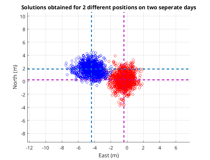 Birds eye view of solutions from both days overlaid with one another
The distance between these two means in the North East plain was 4.3 m. This compares with a real-life measurement of 2.5 m using a tape measure.
Thus the discrepancy between the actual distance and the one measured by the tape measure was 1.8 m.
So, not too bad and I’m quite pleased with the results.
GPS PRN 14 missing from NORAD ephemerides
I was scanning all GPS PRN codes for the recording done at 2020/12/15 at 01:04:57Z and noticed PRN 14 was detectable. I thought this was odd because the Galileo satellite with PRN 14 was also visible in the sky. Looking at Orbitron I noticed for 2020/12/15 at 01:04:57Z the GPS satellite with PRN number 14 was missing. Orbitron uses ephemerides from gps-ops.txt to plot the GPS satellites. This file seems to be obtained from https://www.celestrak.com/NORAD/elements/gps-ops.txt . PRN 14 is missing from this file. Going to Wikipedia and looking at a List of GPS satellites I see that indeed there is a satellite with PRN number 14 and it’s very new and was only launched on the 5th of November. So it looks like NORAD has not added the ephemeris for this new satellite. I thought this was kind of interesting as I accidentally discovered a satellite that I didn’t know was there by doing a brute force search of the PRN codes.
Galileo open service on the E1 band
Galileo is a GNSS run by the European space agency (ESA). They have 3 different bands...
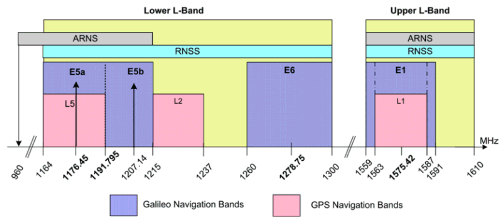 Galileo GNSS bands
You can see that GPS’s L1 band overlaps Galileo’s E1 band. Some of their signals are open to the general public while others are not which they call PRS for the E1 band at least.
Looking through Galileo’s reference documentation webpage, the pdf file called OS SIS ICD v1.3 is the one I want and contains information needed to implement a Galileo receiver the most important being PRN numbers.
I had a look at Galileo Signal Plan for the E1 band...
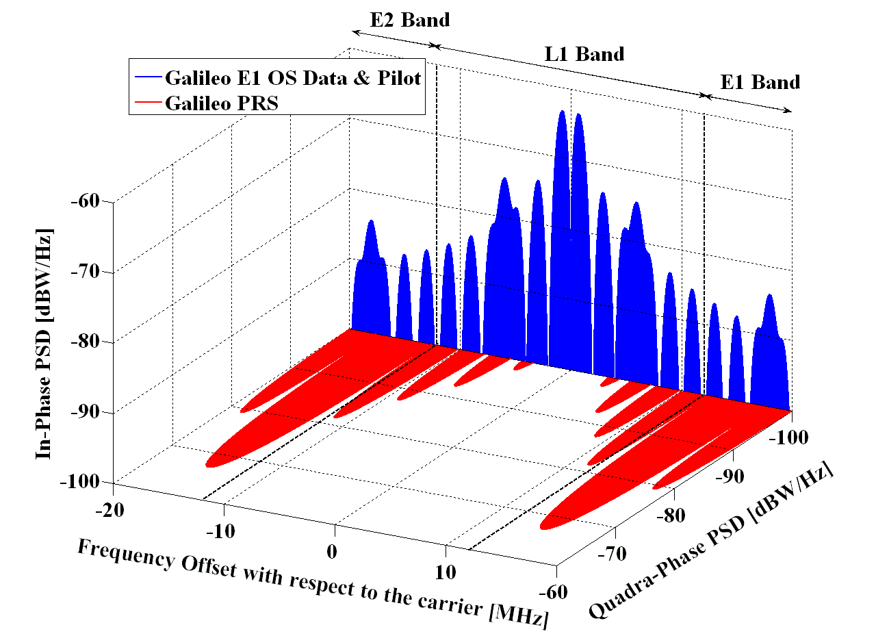 Galileo E1 signal plan
It uses a whopping 32 MHz of bandwidth. I was interested in the E1 open service signal (E1 OS) as that seems to use the smallest bandwidth of any of the Galileo signals and is clearly to allow easy interoperability with current consumer grade GPS receivers. However, the E1 OS signal is still about 24 MHz bandwidth, way more than the 8Ms/s that I have captured my recordings at. However let’s take a closer look.
Galileo signals are weird and initially I was quite intimidated by them. You see mention to things like altBOC, sinBOC, cosBOC, MBOC etc. In the figure below I have put together a block diagram of the E1 OS signal as transmitted by the satellite…
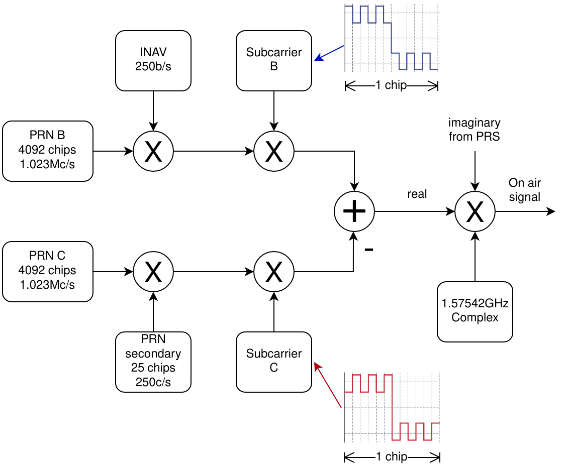 Block diagram of the E1 OS Galileo signal as transmitted by the satellite
All of it’s real except for the last mixing up to RF frequencies where the real is the OS and the imaginary is the PRS signal. The real signal (OS) is the sum of two’s other signals B and C. Signal C is called the pilot signal and just repeats the same thing over and over again with a repeat period of 100 ms. Signal B on the other hand is called the data signal and contains navigation data called INAV.
When receiving the signals you don’t have to use both the B and C signals simply to acquire a signal; using just one will do. PRN B and C are different so for example if you correlate with respect to PRN B, then the pilot’s signal will appear as noise.
The other thing that makes the signals different from legacy GPS are the subcarriers, this is where the BOC comes into it. As you can see from the previous figure the subcarriers are simply repeating squareish waves that are mixed with the chips from the PRNs. These subcarriers are what moves the energy from the center of the carrier frequency towards the side and gives Galileo’s signal plan its distinctive missing center lobe look as you can see from two figures ago.
The two subcarriers are made by adding or subtracting a little of sinBOC(6,1) with sinBOC(1,1), the data subcarrier is sqrt(10/11)sinBOC(1,1)+sqrt(1/11)sinBOC(6,1) while the pilot subcarrier is sqrt(10/11)sinBOC(1,1)-sqrt(1/11)sinBOC(6,1)...
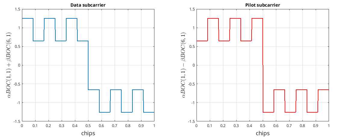 E1 OS subcarriers
In the following figure I plot an example of the real baseband data signal…
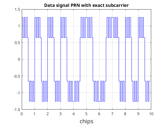 E1 OS baseband data signal example
My sample rate is 8Ms/s, that means 125ns between samples. In either of the subcarriers as described in the previous figure values change every 81ns; that’s faster than my sample rate. I would need a sample rate more like 14Ms/s to describe the subcarriers accurately. So I can’t create the little short pulses you see in the subcarriers. However I can create the general shape of the subcarriers by simply ignoring the high-frequency decorations...
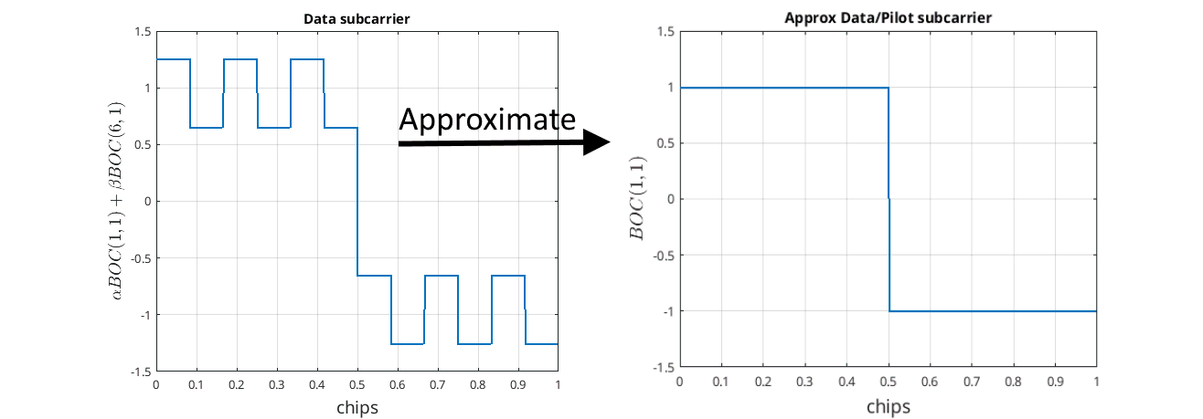 Approximate E1 OS subcarrier from exact subcarrier
If I do this then the subcarrier only changes at twice the speed as that of the chip rate. I can then combine the subcarrier with the PRN to get an apparent chip rate of 2.046Mc/s. Once I’ve done that then the on air signal looks like a BPSK signal mixed with a PRN of length 8184 chips and repeats every 4 ms (8184/2046). If you are screaming out Manchester code; yup I was thinking the same thing. So to a first approximation this E1 OS signal is just Manchester encoding it’s PRN. To be fancy they call this BOC(1,1) and in this particular case sinBOC(1,1). The sin means it looks a little like a sine wave rather than cosine wave. The numbers in this BOC thing are the relative subcarrier frequency and the relative chip frequency respectively, so BOC(1,1) means for every chip there is one rectangular wave, while, BOC(6,1) means every chip there are six waves. If the BOC is not prefixed it seems to imply sine not cosine.
To generate the subcarriers as defined in the SIS ICD document and plot them the following Matlab code can be used...
%create subcarriers
boc11=sign(sin(2*pi*(1/12)*[1:12]));%in binary = 111111000000
boc61=sign(sin(2*pi*(6/12)*[1:12]));%in binary = 101010101010
alpha=sqrt(10/11);
beta=sqrt(1/11);
E1SB=alpha*boc11+beta*boc61;
E1SC=alpha*boc11-beta*boc61;

subplot(1,2,1);
E1SBI=E1SB(floor([1:1/100:13-1/100]));
XI=[1:1/100:13-1/100]-1;
plot(XI/12,E1SBI);
grid on;
xlim([0 1]);
xlabel('chips', 'Fontsize', 14);
ylabel('$\alpha BOC(1,1)+ \beta BOC(6,1) $','Interpreter','latex', 'Fontsize', 14);
title('Data subcarrier');

subplot(1,2,2);
E1SCI=E1SC(floor([1:1/100:13-1/100]));
XI=[1:1/100:13-1/100]-1;
plot(XI/12,E1SCI,'r');
grid on;
xlim([0 1]);
xlabel('chips', 'Fontsize', 14);
ylabel('$\alpha BOC(1,1)- \beta BOC(6,1) $','Interpreter','latex', 'Fontsize', 14);
title('Pilot subcarrier');
While the approximate BOC(1,1)/Manchester subcarrier can be created and plotted using the following Matlab code…
%create Manchester subcarrier
boc11=sign(sin(2*pi*(1/12)*[1:12]));%in binary = 111111000000

E1S_manchesterI=boc11(floor([1:1/100:13-1/100]));
XI=[1:1/100:13-1/100]-1;
figure;
plot(XI/12,E1S_manchesterI);
grid on;
xlim([0 1]);
ylim([-(1.5) (1.5)])
xlabel('chips', 'Fontsize', 14);
ylabel('$BOC(1,1)$','Interpreter','latex', 'Fontsize', 14);
title('Approx Data/Pilot subcarrier');
So using the BOC(1,1)/Manchester approximation effectively we can regard the data or the pilot signal as the following block diagram…
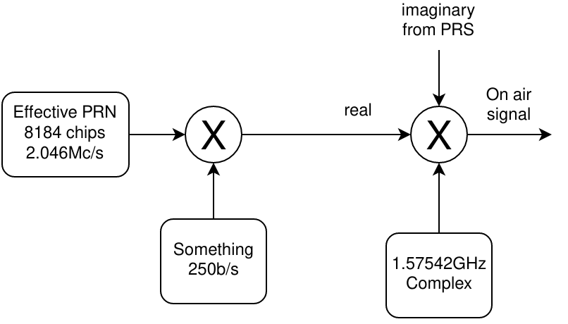 Effectively what the data or pilot signal generation can be approximated as
This looks very similar to what legacy GPS transmits and hence is now relatively easy to acquire and track to get the 250b/s “Something”, be that data or the secondary PRN. This time however there are eight times the number of chips per PRN and the chip rate is twice as fast. One nice difference is there is exactly one PRN per bit compared to legacy GPS where there were 20 PRNs per bit, this means no having to figure out which PRN is the first.
Creating effective Galileo OS E1 PRNs using BOC(1,1) approximation
To create the effect of PRN we first have to figure out what PRN B or PRN C is for the E1 band. In the SIS ICD pdf these numbers are attached and apparently they are just random numbers and I see no mention as to how they were created; here’s one for E1B PRN1 encoded as hexadecimal...
E1B__Code_No_01;F5D710130573541B9DBD4FD9E9B20A0D59D144C54BC7935539D2E75810FB51E494093A0A19DD79C70C5A98E5657AA578097777E86BCC4651CC72F2F974DC766E07AEA3D0B557EF42FF57E6A58E805358CE9257669133B18F80FDBDFB38C5524C7FB1DE079842482990DF58F72321D9201F8979EAB159B2679C9E95AA6D53456C0DF75C2B4316D1E2309216882854253A1FA60CA2C94ECE013E2A8C943341E7D9E5A8464B3AD407E0AE465C3E3DD1BE60A8C3D50F831536401E776BE02A6042FC4A27AF653F0CFC4D4D013F115310788D68CAEAD3ECCCC5330587EB3C22A1459FC8E6FCCE9CDE849A5205E70C6D66D125814D698DD0EEBFEAE52CC65C5C84EEDF207379000E169D318426516AC5D1C31F2E18A65E07AE6E33FDD724B13098B3A444688389EFBBB5EEAB588742BB083B679D42FB26FF77919EAB21DE0389D9997498F967AE05AF0F4C7E177416E18C4D5E6987ED3590690AD127D872F14A8F4903A12329732A9768F82F295BEE391879293E3A97D51435A7F03ED7FBE275F102A83202DC3DE94AF4C712E9D006D182693E9632933E6EB773880CF147B922E74539E4582F79E39723B4C80E42EDCE4C08A8D02221BAE6D17734817D5B531C0D3C1AE723911F3FFF6AAC02E97FEA69E376AF4761E6451CA61FDB2F9187642EFCD63A09AAB680770C1593EEDD4FF4293BFFD6DD2C3367E85B14A654C834B6699421A
Then we have to decode this into 4092 ones and zeros…
111101011101011100010000000100110000010101110011010101000001101110011101101111010100111111011001111010011011001000001010000011010101100111010001010001001100010101001011110001111001001101010101001110011101001011100111010110000001000011111011010100011110010010010100000010010011101000001010000110011101110101111001110001110000110001011010100110001110010101100101011110101010010101111000000010010111011101110111111010000110101111001100010001100101000111001100011100101111001011111001011101001101110001110110011011100000011110101110101000111101000010110101010101111110111101000010111111110101011111100110101001011000111010000000010100110101100011001110100100100101011101100110100100010011001110110001100011111000000011111101101111011111101100111000110001010101001001001100011111111011000111011110000001111001100001000010010010000010100110010000110111110101100011110111001000110010000111011001001000000001111110001001011110011110101010110001010110011011001001100111100111001001111010010101101010100110110101010011010001010110110000001101111101110101110000101011010000110001011011010001111000100011000010010010000101101000100000101000010101000010010100111010000111111010011000001100101000101100100101001110110011100000000100111110001010101000110010010100001100110100000111100111110110011110010110101000010001100100101100111010110101000000011111100000101011100100011001011100001111100011110111010001101111100110000010101000110000111101010100001111100000110001010100110110010000000001111001110111011010111110000000101010011000000100001011111100010010100010011110101111011001010011111100001100111111000100110101001101000000010011111100010001010100110001000001111000100011010110100011001010111010101101001111101100110011001100010100110011000001011000011111101011001111000010001010100001010001011001111111001000111001101111110011001110100111001101111010000100100110100101001000000101111001110000110001101101011001101101000100100101100000010100110101101001100011011101000011101110101111111110101011100101001011001100011001011100010111001000010011101110110111110010000001110011011110010000000000001110000101101001110100110001100001000010011001010001011010101100010111010001110000110001111100101110000110001010011001011110000001111010111001101110001100111111110111010111001001001011000100110000100110001011001110100100010001000110100010000011100010011110111110111011101101011110111010101011010110001000011101000010101110110000100000111011011001111001110101000010111110110010011011111111011101111001000110011110101010110010000111011110000000111000100111011001100110010111010010011000111110010110011110101110000001011010111100001111010011000111111000010111011101000001011011100001100011000100110101011110011010011000011111101101001101011001000001101001000010101101000100100111110110000111001011110001010010101000111101001001000000111010000100100011001010010111001100101010100101110110100011111000001011110010100101011011111011100011100100011000011110010010100100111110001110101001011111010101000101000011010110100111111100000011111011010111111110111110001001110101111100010000001010101000001100100000001011011100001111011110100101001010111101001100011100010010111010011101000000000110110100011000001001101001001111101001011000110010100100110011111001101110101101110111001110001000000011001111000101000111101110010010001011100111010001010011100111100100010110000010111101111001111000111001011100100011101101001100100000001110010000101110110111001110010011000000100010101000110100000010001000100001101110101110011011010001011101110011010010000001011111010101101101010011000111000000110100111100000110101110011100100011100100010001111100111111111111110110101010101100000000101110100101111111111010100110100111100011011101101010111101000111011000011110011001000101000111001010011000011111110110110010111110010001100001110110010000101110111111001101011000111010000010011010101010110110100000000111011100001100000101011001001111101110110111010100111111110100001010010011101111111111110101101101110100101100001100110110011111101000010110110001010010100110010101001100100000110100101101100110100110010100001000011010
Then expand this by 2 times such that 0 becomes 00 and 1 becomes 11, map 0 to -1 and 1 to 1, then alternately multiply by 1 then -1. For brevity I write 1 at + and -1 as - …
+-+-+-+--++--++-+-+--++--++-+-+--+-+-++--+-+-+-+-+-+-++--+-++-+--+-+-+-+-++--++--++-+-+--+-++-+--++--++--++--+-+-+-+-++-+--++-+-+--+-++-+-+--++-+--++-+-+-+--++--++--+-++-+-+-+-+-+--++-+--+-++-+-+-+--++--+-++-+--++-+--+-++--+-+-+-+-++--++--+-+-+-+-++-+--++--++--++-+--+-++-+-+--++--+-+-++--++--+-+-++--+-++-+--+-+-++--++--++--+-++--++-+-+-+--+-+-++-+-+-+--+-++--+-++-+--++--++--++--++--+-++-+-+--+-++-+-+--++--+-++--++-+-+--+-++-+-+--++--++-+--+-+-+-+-+-++--+-+-+-++-+-+-+-+--++-+--++--++--+-+-++-+-+-+--+-++--+-++--+-++--++--+-+-+-+-+-++--+-++--+-++-+-+--++--+-+-+-+-++--++--+-+-+-++-+--+-++-+-+--++-+-+--++--++-+-+-+--+-++-+-+--+-+-++-+-+--+-+-+-++-+--+-+-++--++-+--++--++--+-++-+--+-+-++-+-+--+-++--++--++-+--+-++--++--++-+-+-+--++--++--++--+-++--++--++-+-+-+--+-+-+-+-+-+-++--+-++--++-+-+--++-+-+--++-+-+--++-+-+-+-+-+--++--+-+-+-++-+--++--++-+-+-+--+-++-+--+-+-++--+-+-++-+--+-++--++--+-+-++-+-+--+-++-+--+-+-++-+-+--+-++--++-+-+-+--+-++--++-+-+-+-+--+-++--++-+-+--++--+-++-+--++-+-+--+-+-++-+-+--++-+--+-++-+--++-+-+--+-+-+-+-+-++-+-+-+--++--++-+-+--++--++--+-+-++-+-+-+--++--+-+-+-++--++-+--++--++--++--++--++-+-+-+-+-+--++-+-+-+--++--+-+-+-++--++-+-+-+-+-+-+-+--++--++--++-+-+-+-+-+--+-++-+--++--++--+-++--++-+--+-+-++-+-+--++--+-+-+-+-+-+-+-++--++--+-++-+--++--++-+--+-+-++-+--+-++-+-+--++--+-++--+-++--+-++--++--++-+-+--++-+--+-++-+--++--+-++--+-+-++--+-++-+--+-++-+-+--++-+--+-+-++-+--+-+-++-+-+-+-+--+-+-+-+-+-+-++-+-+-+-+-+--++-+--++-+-+-+--++-+-+-+-+-+--++-+--+-++-+-+--+-+-++-+--+-+-++--++--++--++--+-++--+-++--+-++-+--+-+-++-+-+-+-+-+-+-+--++-+--+-+-++-+-+--++-+-+-+--+-+-+-+-+-++-+-+-+--+-++-+--+-+-+-++--+-+-+-++--+-++--+-++--+-+-+-+-++--++--+-++-+--+-++--+-+-+-++-+--++-+-+-+-+--++--++-+--+-+-++-+-+-+--++-+-+--+-++--+-+-++-+--+-++--+-+-+-++-+-+--++-+--+-++--+-++--+-+-+-+-+-+-+-++-+-+-+-+-+--+-+-++--+-++--++-+-+-+--+-++-+-+-+--++--++--++--++-+--+-+-++--++--++-+--+-++-+--++-+--+-++--+-++-+--+-++-+-+-+--+-++-+-+--+-++--+-++-+-+-+--++--+-++--++--++-+--++--++--++--+-++-+--++-+--++--++--++--+-++-+--++--+-+-++--++--++-+--++-+--+-+-+-+-+-++-+--++-+-+-+-+--++-+-+--++--++-+-+--+-+-+-++--++--++-+--++--+-+-+-++-+--+-+-++--++-+--++-+--++--+-+-++-+-+-+--+-+-++--+-+-++-+--+-+-+-++--+-++--+-++--+-+-+-++--++-+--++--+-+-++--+-+-+-+-++--++--+-+-+-++--++--++--+-+-+-++--+-++--++--+-++-+-+--++--+-+-+-++-+-+-+-+-+--++--+-++-+--+-+-+-+-++-+--+-++--++--+-+-++--++-+--+-++--+-++--++--+-++-+-+--++-+--+-++-+-+--+-+-+-+-+-+-+-++--+-++-+-+-+-+--+-+-++--++--++--++--+-+-++-+--+-++--+-++--++--+-+-+-++-+--+-++-+--++--+-+-+-+-++-+-+-+--+-++-+-+-+-+--++-+--+-++-+-+-+--+-++--++-+--++--++--+-+-+-++--+-+-++-+--+-++--+-++--++-+--+-++-+-+--++--++-+--++--++--+-+-+-+-+-+-++-+-+-+-+-+--+-+-+-+-++--++--++-+-+--+-++--+-+-++-+--+-++--++-+-+--+-+-+-++-+-+-+-+--+-+-++-+-+-+--++-+-+--++--+-+-++-+--++-+-+-+-+--+-++-+--+-+-+-+-++--++--++--+-+-++-+--+-+-+-++-+-+-+--++--++--++--+-+-+-++-+-+-+-+--+-+-+-+-++-+--+-+-++--++--++--+-++-+--++-+--+-++--+-+-+-+-+-+-+-+-++-+-+-+--+-++-+-+--++-+-+--++-+--++--++-+-+-+-+--+-+-+-+-+-+-++--++--++--+-++-+--+-+-+-+-+-++--+-+-+-++--++-+-+-+-+-+--+-+-++--+-++--++--+-+-++--+-++-+-+-+--++--++-+-+-+--++-+--+-++--++--+-++-+-+-+-+-+--+-+-+-++-+--+-++-+-+-+-+-+--+-+-++--+-++-+--++--++--+-++-+--++--+-+-+-+-+-+-++--+-++-+-+-+-+-+--+-+-++--+-+-++--++--++--+-++-+--+-+-++--+-+-+-+-++-+-+-+--+-+-++--+-+-++-+--++--++-+--++--+-+-++-+--+-++--++--++-+-+--++--++--++-+--++--+-++-+-+-+-+--++-+--+-++-+--+-++-+--+-++-+--+-+-++--++--+-++-+--+-++-+--+-+-+-+-++--++-+--+-+-+-++-+-+-+-+-+--++--++-+--+-++-+-+-+--+-+-+-++--+-+-++--++--++--+-+-+-++--++--+-+-++--++-+--+-++-+-+-+-+-+-+--+-++--+-+-++-+-+--+-++-+--++-+-+-+-+-+--+-++-+--+-++-+-+--++--+-++-+-+--+-++-+--++-+-+-+--++--+-+-+-++--+-++--+-++-+--++--+-++--++--+-++--+-+-+-+-+-++--++-+-+-+--+-++-+-+--+-+-+-++-+--+-+-++-+--++-+--++--++-+--+-++-+--++-+--++--+-+-++--+-++--+-++--++-+--+-+-+-+-+-++--++--+-++-+--++--++-+--++--+-++-+--+-+-++-+--++-+-+--++--+-+-+-++-+-+--++-+-+--++--++-+-+-+-+-+-+-+-+--++--++--++-+-+--+-++--++--+-++--++-+--+-++-+--+-+-++-+--+-++--++-+-+--+-+-++--++-+-+--+-++--+-+-+-++--+-++-+-+--++-+-+--++-+--++-+-+-+-+--+-++--+-+-+-+-+-++-+-+--+-++-+--++-+-+-+--+-++--+-+-+-+-+-+-+-+-+-+-+-++-+-+--+-+-+-++--++-+--++--+-++-+-+--++--+-++-+--+-+-++-+--+-+-+-++--+-+-+-++--+-++-+--+-++--++--+-+-++--++-+--++--++--++-+--+-+-++--++-+-+--++--+-+-++-+-+--+-+-+-++-+--+-+-++-+-+-+-+--+-++--++-+-+--+-+-+-++-+--+-+-++--++--+-++-+--+-++--++-+-+-+--+-+-+-+-+-++-+-+-+--++--++-+-+--+-++-+--++-+-+--+-+-++-+--+-++-+-+-+-+-+-+-+--++-+-+--++--++-+-+--+-++--+-++--+-++--++-+--+-+-++--+-++-+--+-+-+-++--+-++-+--+-+-++--++-+--+-++-+-+--++--+-++--+-+-++--+-+-++--+-+-++-+--++--+-+-++--+-+-+-+-++-+-+--+-+-++--+-++-+-+-+--++-+-+-+-+--++-+-+--++-+-+--++-+--++--++-+-+-+--++-+-+--++--++--++--++-+--++--++-+--+-+-++--+-+-+-++-+-+--++--+-+-+-++--++--++-+-+--++-+--+-+-+-++--+-+-+-+-++-+-+--++-+--++-+--+-++-+-+-+--+-++-+-+--++--++--+-+-+-++--++-+-+-+-+--++-+--+-++--+-++-+--++-+-+-+-+-+-+-+--++-+-+--++-+-+-+--+-++--+-+-++-+--+-++-+-+-+--++--++--++--++-+--+-++--+-+-+-++-+-+--++-+-+-+--+-+-+-+-+-+-++-+-+--+-+-++--+-++-+-+--++-+--+-++-+--+-++-+--+-++--++-+-+--++--+-++--+-++-+--+-+-++-+-+-+-+--+-++--++-+--+-++-+-+-+--++--++-+-+--+-+-+-+-+-++--++-+--++--++-+-+-+--+-+-+-++-+-+-+--++--+-++-+--+-+-++-+-+-+-+-+--+-+-+-++--++-+-+--++-+-+--++--+-+-+-+-++--++-+--++-+-+--+-+-+-++-+--+-+-++-+--+-+-++--+-++-+--++--++--++-+-+-+--+-++-+--++--+-++-+--+-+-+-++-+-+-+-+-+--++-+--++--+-++-+--++--++-+--+-++--+-+-+-+-++-+--++--+-++--+-+-+-++--++--++-+--++--+-+-++--+-++--+-++-+-+-+-+--++-+--+-+-+-++-+-+--+-++--++-+-+-+--+-+-++--++--+-++--++--++--+-+-++-+-+-+--++--+-++--+-++--+-+-+-+-+-++-+-+--++--+-+-+-++--+-++--+-+-++-+--+-++--++--+-++--++-+-+--+-++-+--+-++--++--++--++--+-++--++-+-+--++-+--++--+-+-++-+-+-+-+--+-+-+-+-++--++-+-+-+--+-++--++--+-++--++--++-+--++-+-+-+-+--++-+-+--+-+-++-+-+--+-++--+-+-++-+--+-+-+-++-+-+-+--+-++--+-++--++--+-++--+-++-+-+-+-+--+-+-++-+-+--++--++--+-++--++-+-+-+-+--++--++--++--+-+-++--++--+-+-+-++-+--++--++-+--++--+-++-+-+-+-+-+-+--+-+-+-+-+-++-+-+-+-+--++-+--++--++-+-+-+-+-+-+-+--++-+-+-+-+--+-+-++--+-++-+-+--++--++-+-+-+-+--+-+-++--+-+-+-+-+-++--++--++--++--+-+-+-+-++-+--+-++--+-+-+-+-+-+-++--++-+--++-+-+--+-+-+-++-+-+-+--++-+-+-+--++--+-++--++--+-++--++--++-+-+-+--++--+-++-+--+-+-++-+-+--+-+-++--+-++--++-+-+--++--+-++-+-+--++--+-+-+-+-+-+-+-+-++-+--++-+--++--+-+-++-+--+-+-+-+-++--+-++-+--++--+-++--+-++-+-+-+-+--++--+-++--++-+--+-+-++-+--+-++--++--+-++--+-++-+--+-++-+-+-+-+--+-++-+--++-+-+--++--++-+--++-+-+--++-+-+--+-++-+-+--+-+-++--+-+-+-+-+-+-++-+--+-++-+-+-+--+-+-++--++--+-+-++-+-+-+--++-+-+--+-++--+-++--+-+-++--++-+-+--+-++-+-+--++--+-+-++--++--+-++-+-+--+-++-+-+-+--+-++--+-+-++--++-+--+-+-+-+-++--++-+-+-+--++-+-+-+--+-++-+-+-+--+-+-++-+-+--+-++--++-+-+--+-++--+-+-++-+-+--++-+--++--+-++-+--+-++--+-+-+-+-+-+-++-+-+--+-++--+-+-+-++--++-+-+--++-+--++-+-+--+-++-+-+--+-++--+-++-+--+-+-+-+-+-++--+-+-++--++--++--+-+-++-+--++--+-+-+-+-+-++--+-+-++--+-+-++--+-+-+-++-+--++-+-+--++--++-+-+--+-++-+--++-+--++--+-+-++--++-+-+--++-+-+--+-++-+--++--+-++--+-+-+-+-+-++--++-+-+-+-+--++--++--++-+--++-+--++--++--+-++-+--+-+-++-+-+--+-+-+-+-+-++-+--++--+-++-+-+-+--+-+-+-+-++-+--++--++-+-+--+-++-+-+--+-++--+-+-++-+-+--+-++--+-+-++--+-+-++-+-+-+-+--+-++-+-+-+-+-+-+-+-+-+-+-+-+-+--++-+--++--++--++--++--++-+--+-+-+-+-+-+-+-++--++-+-+--++--+-++--++-+-+-+-+-+-+-+-+-+--++--++--+-++-+--++--+-++-+-+-+--+-+-++-+--++-+-+--++-+--++--++--++-+-+-+--++--+-+-++-+-+--++-+--+-+-+-++-+-+-+--+-++-+--+-++--+-+-++--++--+-+-++-+-+--+-++--++--+-++-+--+-+-+-++-+-+-+-+-+-+--++-+--++-+--+-++--++-+-+-+-+--+-++--+-+-++-+--+-+-+-++-+-+--++-+--+-++--+-+-+-++--++-+-+--++-+-+-+-+-+--+-++-+--++--++-+--+-+-++-+-+--++--+-+-+-+-++--+-++-+--++--++--++--++--++-+--++-+--++--+-+-+-+-+-+-+-++-+-+--++-+-+--+-+-+-++-+--+-+-+-+-++--++--++-+--+-++--+-++-+-+-+-+--++-+-+--++-+--++-+-+--++--++--+-++-+-+-+-+-+-+-+--++--+-+-+-++--++--+-++--+-++-+-+--++-+-+-+-+-+-+-+-+-+-+-+--++--++-+--++-+--++-+-+--++--+-++--++-+--+-+-+-++-+--+-++-+--++-+--+-++-+-+-+-+-+--++--+-+-+-++--++-+--++-+--+-+-++--++--+-++--++--+-++-+--+-++--++--++--+-++-+--+-++--+-+-+-+-++-+--++--+-++--++-+--++-+--+-++-+--++--+-++-+--+-++--++--+-+-+-++--+-+-+-++-+--++--+
That's a lots of bits. However I found GNSScodegen.m that already generates PRN codes for Galileo, then the code for generating these effective PRN codes is as this simple as…
%create primary codes
C=GNSScodegen(sv,'E1C');%4092 chips
B=GNSScodegen(sv,'E1B');%4092 chips

%Then something to create the BOC(1,1) code…
boc11=sign(sin(2*pi*(1/2)*[1:2]));

%Expand the PRNs so each chip takes 2 samples…
B2=repelem(B,2);
C2=repelem(C,2);

%Repeat the BOC(1,1) code so it’s the same length as B2 and C2…
boc11_12=repmat(boc11,[1,numel(B)]);

%And finally mix the BOC(1,1) subcarrier with the PRNs…
prn_data=(B2.*boc11_12)';%8184 chips
prn_pilot=(C2.*boc11_12)';%8184 chips
I took the previous code I wrote for the GPS and modified it a bit so you can select either GPS or Galileo for the PRN NCO. The rest of the tracking code is basically the same. Testing this out about the following points at 250c/s for the pilot signal...
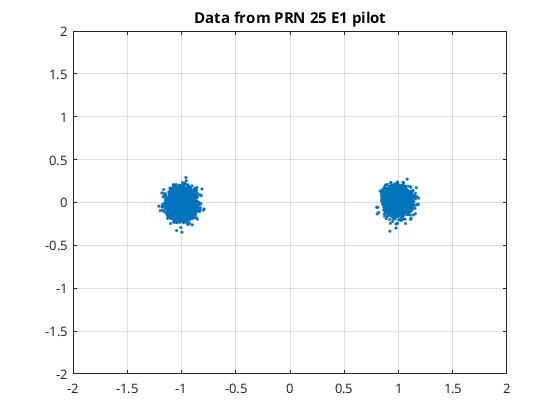 Points from the 250c/s pilot secondary PRN
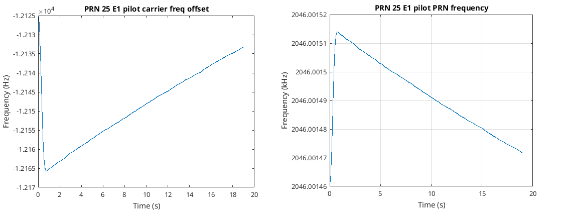 Tracking frequencies
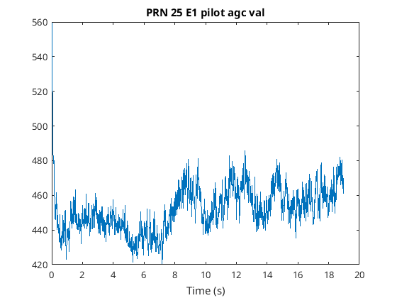 AGC
AGC
The PRN frequency and the carrier frequency don’t go in the same direction probably because I’ve mucked up the rotation of the NCO which happens. However it doesn’t matter.
Secondary PRN
The pilot signal outputs a secondary PRN of length 25 at 250 secondly PRNs per second. According to the SIS ICD pdf it should be the sequence 0011100000001010110110010. I then plotted the demodulated signal and a scanning manner such that only 25 values could be plotted per line and increased the vertical offset for each scan line...
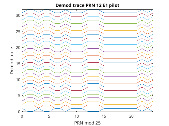 Pilot demod trace wrapped to 25 bits
As you can see by the third scan line each one was identical. This means indeed there is a code that repeats every 25 demodulated symbols. However, strangely enough this didn’t work for all satellites; here is the output for PRN 2...
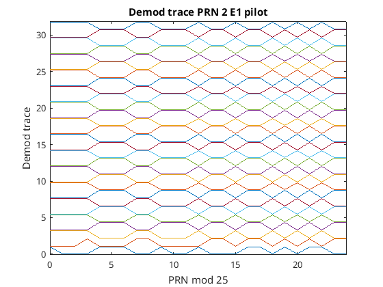 Pilot demod trace not repeating every 25 bits. Why?
This pattern repeats every 50 bits and is unexpected. I’m not sure why this is happening to some satellites yet. What is happening though is that every alternate bit is getting flipped. To show this I fliped every alternate bit...
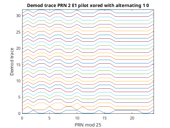 Alternate bit flips make the pattern repeat as it should
I'll get back to this problem later.
I then added some extra code to find the secondary PRN code alignment...
%find pilot signal and align and invert if needed
number_of_start_bits_to_search=150;
assert(((number_of_start_bits_to_search-1)+250)<=numel(rx_data),'not enough demodulated bits\n');
secondary_prn=[0 0 1 1 1 0 0 0 0 0 0 0 1 0 1 0 1 1 0 1 1 0 0 1 0 ]';%CS25
secondary_prn=repmat(secondary_prn,[1,10]);
val_min=inf;
val_max=-inf;
min_loc=-1;
max_loc=-1;
for k=1:number_of_start_bits_to_search
    tmp=reshape(rx_data(k:((k-1)+250)),[25,10]);
    val=sum(sum(bitxor(secondary_prn,tmp))/250);
    if(val<val_min)
        val_min=val;
        min_loc=k;
    end
    if(val>val_max)
        val_max=val;
        max_loc=k;
    end
end
if((1-val_max)<val_min)
    fprintf('inverted signal\n');
    rx_data=1-rx_data;
    loc=max_loc;
else
    loc=min_loc;
end
loc=mod(loc-1,25)+1;
rx_data=rx_data(loc:end);
Now the output has the correct bit alignment…
0011011100000101110111101
1011100011110101001010010
0011100000001010110110010
0011100000001010110110010
0011100000001010110110010
You can see it’s not until the third secondary PRN that the signal matches the expected secondary PRN of 0011100000001010110110010
Wrong locking frequency issue
That I’ve seen some satellites produce a secondary PRN that repeats every 50 bits rather than 25 bits says that something is wrong and needs to be figured out.
I looked at PRN 24 E1 OS from the very first recording I made on 2020/10/25 which is quite a poor recording with drop USB frames. The drop frames cause reacquisition to happen. During one of these reacquisition’s I was lucky enough to see the following figures...
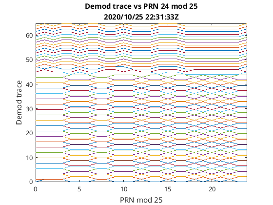 Relocking causes change from 50bit repeat period to 25bit repeat period
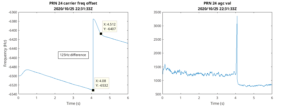 Two distinct frequency locks and different AGC gains before and after relocking
Here you can see reacquisition happened around four seconds. The secondary PRN went from repeating every 50 to every 25 demodulated bits, while the carrier frequency changed by approximately 125 Hz, and the AGC gain went down a bit. The AGC dropping is a sign that correlation has improved after reacquisition. The 125 Hz carrier change is interesting as this is half the secondary PRN rate. All three of these figures suggest that there are stable sub optimal tracking locations for the tracking loop I created which is not good.
So I then had a look at the autocorrelation using just PRNs, PRNs with a BOC(1,1) subcarrier and PRNs with a BOC(1,1)-BOC(6,1)...
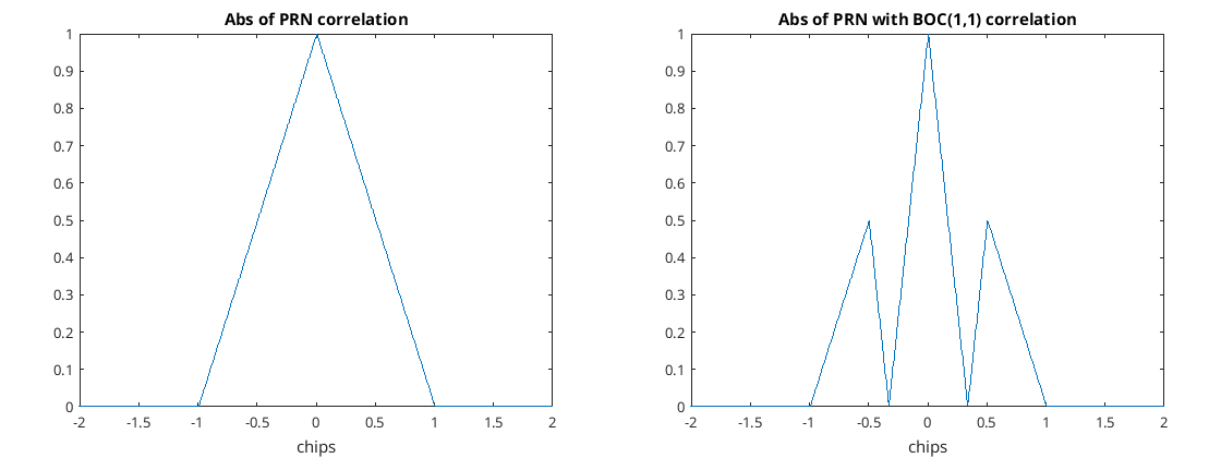 Correlation of a PRN and a PRN mixed with a BOC(1,1) subcarrier
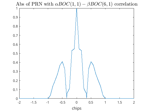 Correlation of a PRN mixed with an alpha*BOC(1,1)-beta*BOC(6,1) subcarrier
These graphs are produced using the following code...
expand_factor=100;
C=GNSScodegen(sv,'E1C');
prn_data=repelem(C,2*expand_factor);
offset=numel(prn_data)/2;
cB=conj(fft(prn_data));
prn_data=circshift( prn_data,offset );
A=fft(prn_data);
circcorr_xy = ifft(A.*cB);
circcorr_xy=circcorr_xy./max(circcorr_xy);
plot([1-offset:numel(circcorr_xy)-offset]./(2*expand_factor),abs(circcorr_xy));
xlim([-2 2]);
title('Abs of PRN correlation');
xlabel('chips');

expand_factor=100;
C=GNSScodegen(sv,'E1C');
boc11=sign(sin(2*pi*(1/(expand_factor*2))*[1:(expand_factor*2)]-(1/(expand_factor*2))));
C2=repelem(C,numel(boc11));
boc11_2expand_factor=repmat(boc11,[1,numel(C)]);
prn_data=(C2.*boc11_2expand_factor)';
offset=numel(prn_data)/2;
cB=conj(fft(prn_data));
prn_data=circshift( prn_data,offset );
A=fft(prn_data);
circcorr_xy = ifft(A.*cB);
circcorr_xy=circcorr_xy./max(circcorr_xy);
figure;
plot([1-offset:numel(circcorr_xy)-offset]./(2*expand_factor),abs(circcorr_xy));
xlim([-2 2]);
title('Abs of PRN with BOC(1,1) correlation');
xlabel('chips');

expand_factor=900;
C=GNSScodegen(sv,'E1C');
boc11=sign(sin(2*pi*(1/(expand_factor*2))*[1:(expand_factor*2)]-(1/(expand_factor*2))));
boc61=sign(sin(2*pi*(6/(expand_factor*2))*[1:(expand_factor*2)]-(1/(expand_factor*2))));
alpha=sqrt(10/11);
beta=sqrt(1/11);
CSub=alpha*boc11-beta*boc61;
C2=repelem(C,numel(CSub));
CSub_2expand_factor=repmat(CSub,[1,numel(C)]);
prn_data=(C2.*CSub_2expand_factor)';
offset=numel(prn_data)/2;
cB=conj(fft(prn_data));
prn_data=circshift( prn_data,offset );
A=fft(prn_data);
circcorr_xy = ifft(A.*cB);
circcorr_xy=circcorr_xy./max(circcorr_xy);
figure;
plot([1-offset:numel(circcorr_xy)-offset]./(2*expand_factor),abs(circcorr_xy));
xlim([-2 2]);
title('Abs of PRN with $\alpha BOC(1,1)- \beta BOC(6,1)$ correlation','Interpreter','latex','fontsize',14);
xlabel('chips');
I also had a look at the real life correlation I was doing with PRN 24...
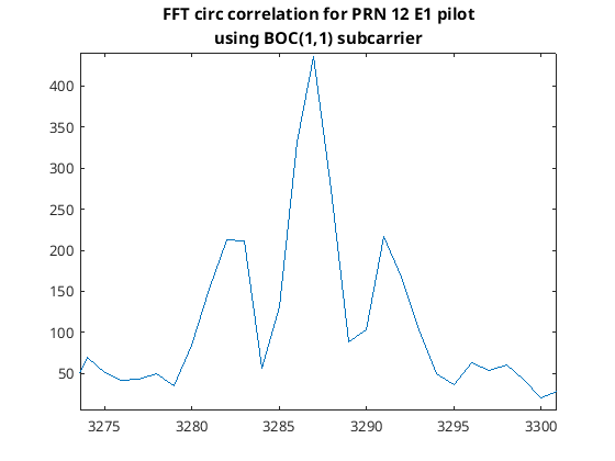 Real life coarse acquisition correlation chip axis
So when using these subcarriers you get 2 pesky peaks to each side of the main peak. For the simple BOC(1,1) I’m using these peaks are 50% of that of the main peak and it’s quite conceivable that the tracking algorithm will lock onto these peaks. The lower value of these peaks would explain the change of the AGC gain during reacquisition as correlation is inversely proportional to AGC gain. However, I’m still not sure how these peaks might affect the carrier frequency tracking and the alternate flipping of the demodulated data. I then looked around the correlation with respect to the prompt correlation during the chip tracking algorithm for the incorrect data pattern that repeats every 50 bits...
As can be seen in this case the algorithm is locked to the correct peak even though the data pattern is incorrect. So even though I could accidentally lock onto one of these smaller peaks it’s not the reason why I’m getting the incorrect data pattern and the incorrect carrier frequency. It really does look as if the carrier frequency is incorrect and that is causing the 180° rotation (or some odd multiple thereof) every bit; the question is why?
Let’s have a look at the result from the coarse acquisition of carrier frequency using the FFT. I put in some code into the FFT acquisition class so could draw me a plot of the frequency domain for the best chip correlation. On this figure I marked the maximum frequency which it locked onto but also the frequency it should have outputted...
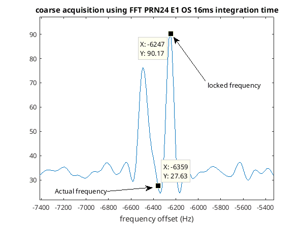 Real life coarse acquisition correlation frequency axis
This was for a Galileo satellite that caused the incorrect 50 bit repeat period. You can see two peaks rather than the expected single peak. I assume this is because I have crossed a bit boundary. Anyway this shows that the coarse acquisition code might be a few hundred hertz out. The way I then measure the frequency more accurately in the tracking code is to look how far a point has moved between PRNs (I ignore 180° rotations). For GPS there are 1000 PRNs per second. So for GPS the fine frequency tracking can lock onto the correct frequency even when the frequency is out by as much as 250Hz. For Galileo however there are only 250 PRNs per second so the fine frequency tracking can only lock onto a signal correctly if it’s less than 62.5 Hz out. That’s the problem, 62.5 Hz is not enough when the coarse acquisition may output frequency that is 200 Hz out. So let’s fix it.
To fix it it was as simple as the following three lines...
fast_points=agc.agc_val*sum(reshape(a_slow_spinning.*prn_nco.block,[samples_per_correlation/(sub_sample_factor*prns_per_correlation),(sub_sample_factor*prns_per_correlation)]))/(samples_per_correlation/(sub_sample_factor*prns_per_correlation));
fast_points=carrier_tracker_fast_points.update(fast_points);
carrier_tracker.frequency_offset=carrier_tracker_fast_points.frequency_offset;
What this does is simply split up the incoming signal with the PRN into smaller blocks than a single PRN then estimates the frequency based on these points. sub_sample_factor is the number of these smaller blocks that make up the PRN. So sub_sample_factor=4 for Galileo implies a thousand of these sub blocks a second and thus allow it to lock onto frequencies that are out by as much as 250Hz, the same as GPS.
Running this new code on the signal from the bad day that would initially lock onto the wrong frequency then lock onto the correct frequency I got the following demodulation trace...
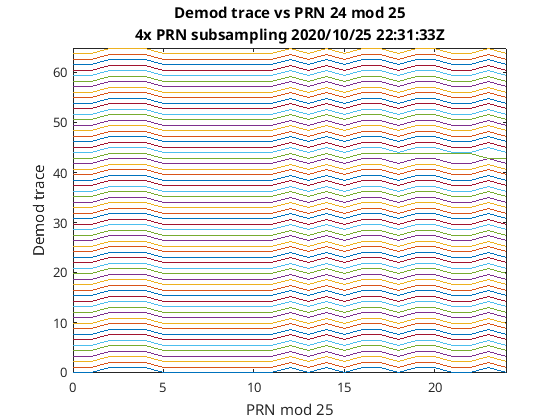 Pilot demod trace with wrong carrier frequency issue solved
This time it’s almost perfect even the re-locking barely affected the demodulation. The repeat period is 25 which is expected. The frequency tracking can be seen in the following figure...
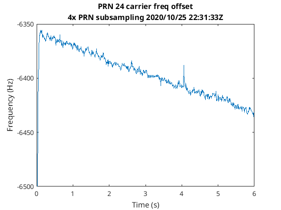 Carrier frequency now locking onto the correct frequency
You can see it adjusted the frequency by about 150 Hz after the coarse acquisition. So yay I think I have fixed that problem. Initially I thought it might’ve been the BOC(1,1) correlation but in the end it turned out simply that I wasn’t sampling the output fast enough so was getting rotation aliasing. That’s debugging for you, sometimes go down wrong paths.
Have you heard of PRN 33 and 36?
The SIS ICD pdf says that satellites with SVIDs of 1 to 36 are assigned corresponding primary PRN numbers from 1 to 36 (3.6.1). It doesn’t mention satellites 37 to 50 and I have not seen these in Orbitron. Orbitron does however mention PRN 33 and 36. In fact for the current signal I’m using PRN 36 is pretty much above my head
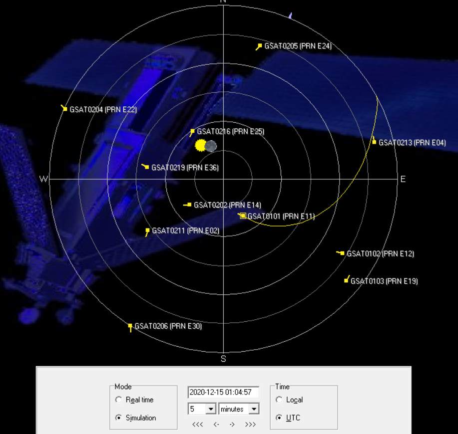 Orbitron PRN36???
However this is not a satellite I can detect even though it should be very strong given the recording quality and the elevation of the satellite.
In addition when I made the first recording (2020/10/25 22:31:31Z), according to Orbitron PRN 33 was in the sky but I was unable to detect that PRN as well. However this recording was of poorer quality.
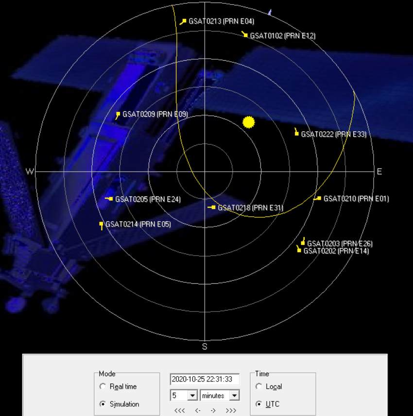 Orbitron PRN33???
I tried both the pilot and the data PRNs for both PRN 33 and PRN 36, and nothing.
So what’s the story here? Were these two satellites not working at the time? Are Orbitron’s ephemerides wrong? Are the PRN numbers for the satellites correct? I just don’t know, it’s a bit of a mystery.
In Octave
Octave is an open source cross-platform version of Matlab and can be downloaded from https://www.gnu.org/software/octave/download .
I installed it on my Windows computer and tested out with the tracking code that I wrote and with just two tiny changes it worked bar the PRN chip frequency graph...
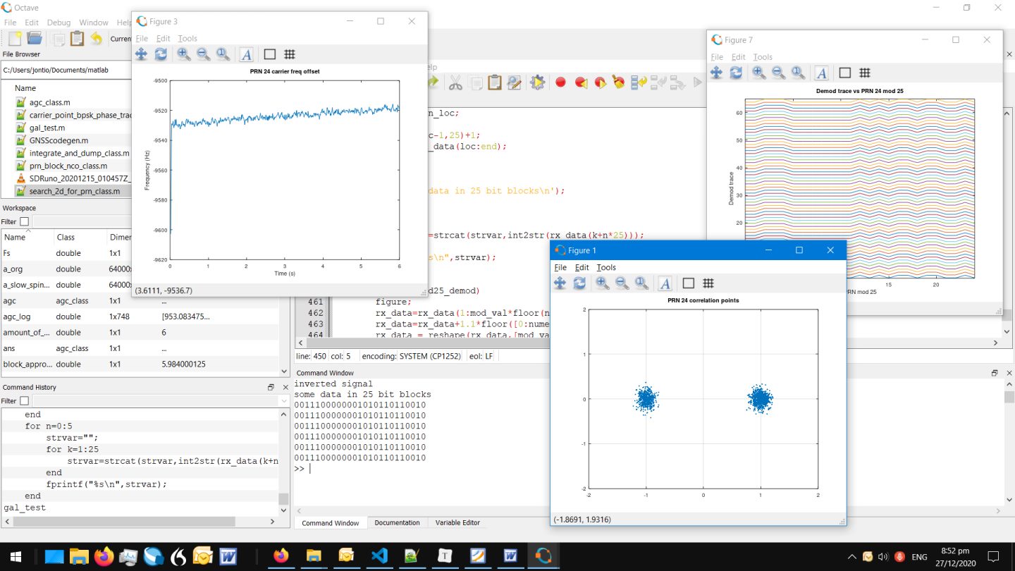 Tracking Galileo satellite using Octave
Here is the code I used to detect the GPS and Galileo satellites which will run in Octave. It contains a 1 second real life recording of the L1/E1 band so you can experement searching for satellites and also tracking the signals of them. You should be able to run it in Linux or Windows.
For those who want to have a go at decoding the INAV navigation data here is about 12 seconds of PRN 24; it may or may not be inverted...
10010011011111101001010000101001000111111000011111010101011100000100111000000000
01001111100111011000011110100100100000100101010100111110101110110111111111100110
00000000001100000010010010011100000001100110100111011110100011111001110100001011
00000001100000000000000000000001000110111111111111111111111110011001011111111111
11111111110101011100000000000000000000001011000110000000000000000000001101111011
11111111111111111111110000000111111111111111111111001101111000000000000000000000
10101010110000010011100000110101111011010100001011111000000010000110101101010111
11111010000000000101010011111100000100010111100010101000001010011010110111110001
11110111110100010010100001111111100000010100001111000001100110001001000101011111
11111000101110001011000000011000000000000000000000010001101111111111111111111111
10011001011111111111111111111101010111000000000000000000000010110001100000000000
00000000001101111011111111111111111111111100000001111111111111111111110011011110
00000000000000000000101010101100000100101100011011111110000111000010101000001111
00000100101101010110001011111000000010001100111111011101000101111001000110000011
10101000110111110101111101111011101010011000011011010000000011010101100000010010
00101001011010011101111110010110000010110000000100101011101111001010000010111100
10000011111011001010110100010000000001001000100000011001101010100110010011000101
11000001011111110110110110110111101110001010001001011000110000111010110000111111
11010101000011110111011101010100111001001000001011000001100111110010100111101001
11000001110100100100100001111000110100001101010111000000010011101100001101011111
01111011100010001011011111010001111011111001011010110001100110000000000000000110
10011101010000000011010010100010100010111111100011001000101100000000101100001101
10010011111100011010001011010100011011111110100000111000110100110010010000011110
00100010100011100111110100110011010110011001001101100011000100001011101110111110
01110000111111111000101011100100110100100010111001011100011111101010110000011000
10010100111111101100111000100010100000111000010001011101110010101010011000001000
00001110011011101101011110101011100100111000000110111110010010110011011010010110
10000001011100000101000001010110000111101110111001001100100101111110001000001011
00000000011000110100011011010011011110101101010100011000010000100011110101100011
11011100001100010010010101011110111001100011001111101001001000111101010110111101
11001110101000001111100100001111001001100110110000100101111011111001000101010111
00111010110000010111111101110001111000010110001000010111010100000100101101010000
00111001001000000001001011111110111001111111101001000000111110110110100111111111
00110100000101100001100001100010000000001100011111000001110100101011110101000111
11111010100100001011000000011000000000000000000000010001101111111111111111111111
10011001011111111111111111111101010111000000000000000000000010110001100000000000
00000000001101111011111111111111111111111100000001111111111111111111110011011110
Jonti 2020
Home